Here is another way to represent this.
domain = Range[-5, 10, 0.1];
sols1 = Table[5 Surd[ x, 3]^2 - Surd[x, 3]^5, {x, -5, 10, 0.1}];
sols2 = Table[5 x^(2/3) - x^(5/3), {x, -5, 10, 0.1}];
sols3 = Conjugate /@ sols2;
ListPointPlot3D[{Flatten /@
  Transpose[{domain, {Re[#], Im[#]} & /@ sols2}],
  Flatten /@ Transpose[{domain, {Re[#], Im[#]} & /@ sols3}],
  Flatten /@ Transpose[{domain, {Re[#], Im[#]} & /@ sols1}]},
 AspectRatio -> 1, AxesLabel -> {"x-Axis", "real", "imaginary"},
 LabelStyle -> Directive[Bold, Medium]]
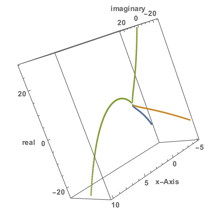
The domain-variable just is input to our function. sols1 computes the real-values of the root (green curve in the picture). sols2 and sols3 are the principal (complex) solutions to the roots together with the conjugate complex solutions. Because the roots of negative numbers are not unique in general, we can get more than one "solution". If other pieces of software assume that we want only the real roots, they do not have issues with this, but do make some potentially critical assumptions that we might not want to make.
Cheers,
M.
PS: The figure is actually not easy to read this way. It shows how much better it is to have Mathematic than a static document. If you take compute it and rotate it, it becomes much clearer.
PPS: If you dislike the awkward way of plotting the lists of points you can, of course, also use ParametricPlot3D
Show[ParametricPlot3D[{x, Re[5 x^(2/3) - x^(5/3)],
   Im[5 x^(2/3) - x^(5/3)]}, {x, -5, 10}, AspectRatio -> 1,
  PlotStyle -> Red, PlotRange -> {{-5, 10}, {-20, 20}, {-20, 20}}],
 ParametricPlot3D[{x,
   Re[5 x^(2/3) - x^(5/3)], -Im[5 x^(2/3) - x^(5/3)]}, {x, -5, 10},
  AspectRatio -> 1, PlotStyle -> Red],
 ParametricPlot3D[{x, Re[5 Surd[x, 3]^2 - Surd[x, 3]^5],
   Im[5 Surd[ x, 3]^2 - Surd[x, 3]^5]}, {x, -5, 10}]]
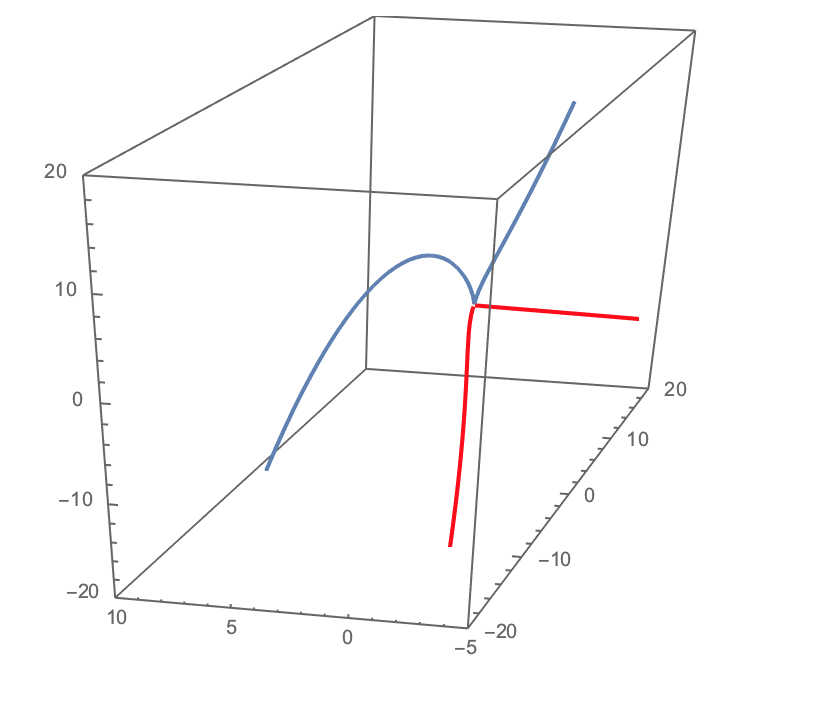
The blue line is the "real" solution and the other two correspond to "complex and conjugate complex solutions".


