Hi Muhammad,

I am no quite sure whether this is what you want to achieve, but one way is to define the following two functions;

cartesianToPolarEqn[eqn_] := 
 Module[{}, eqn /. {Rule @@@ Transpose@{{x, y}, FromPolarCoordinates[{r, \[Phi]}]}}]

and

implicitPolarPlot[eqn_, options : OptionsPattern[]] := Module[{},pl = ContourPlot[eqn, {r, 0, 8 Pi}, {\[Phi], 0, 2 Pi}, 
PlotPoints -> 100]; g[r_, th_] := {r Cos[th], r Sin[th]};pl[[1, 1]] = g @@@ pl[[1, 1]]; Show[pl, options]]

If you then want to convert your implicit equation into polar coordinates you can do:

cartesianToPolarEqn[(x/a)^2 + (y/b)^2 == 1 ]

which gives:

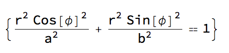
You can then generate a plot of this using:

implicitPolarPlot[(r^2 Cos[\[Phi]]^2)/a^2 + (r^2 Sin[\[Phi]]^2)/b^2 ==1 /. {a -> 1, b -> 2}]

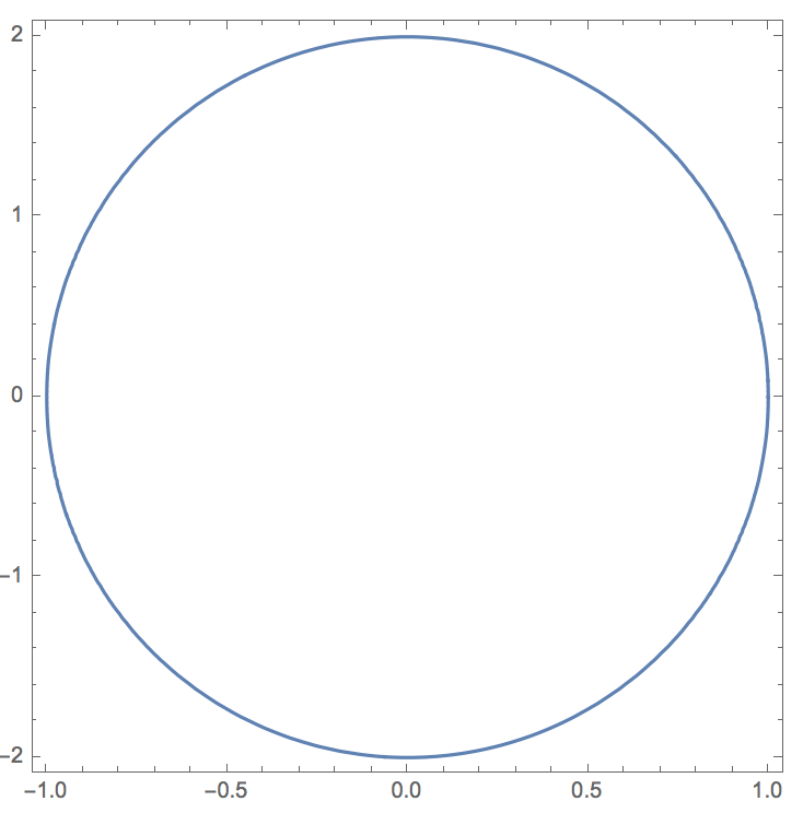
This rescales the axes so that everything looks circular again, but the function also takes additional arguments such that

implicitPolarPlot[(r^2 Cos[\[Phi]]^2)/a^2 + (r^2 Sin[\[Phi]]^2)/b^2 ==1 /. {a -> 1, b -> 2}, PlotRange -> {{-2, 2}, {-2, 2}}]

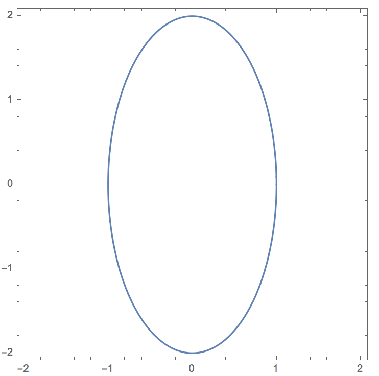
Note that in both cases I needed to specify the parameters "a" and "b".

Cheers,

Marco

of course one does not have to go back and forth polar coordinates if one has the equation in cartesian coordinates:

equation=(x/a)^2+(y/b)^2==1;
equation=equation/.{a->2,b->3}

plot=ContourPlot[Evaluate[equation],{x,-6,6},{y,-6,6},PlotPoints->100];
lines=Cases[Normal[plot],Line[_],\[Infinity]];
max=Max[Cases[lines,(x:{_?NumericQ,_?NumericQ}):>Norm[x],\[Infinity]]];
PolarPlot[1.2max,{\[Phi],0,2\[Pi]},Epilog->lines,PlotStyle->None,PlotRange->5,PolarAxes->Automatic,PolarTicks->{"Degrees",Automatic}]

giving the same plot...