2D cylindrical mirror anamorphosis is well known and in the past, I made several Wolfram Demonstrations on the subject. Such as : Cylindrical Mirror Anamorphosis and Cylindrical Anamorphosis of Some Popular Images,
George Beck of Wolfram Research drew my attention to the website of the London artist Jonty Hurwitz: Wild New Anamorphic Sculptures From the Warped Mind of Jonty Hurwitz. And I went on to see what could be done using the Graphic capabilities of Mathematica...
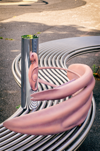
These sculptures are cases of 3D mirror or catoptric anamorphosis in contrast with its counterpart, perspective or oblique anamorphosis .
We first need to look at the geometry of the setup for cylindrical mirror anamorphosis: A deformed 3D image (sculpture) is resting on the x-y plane, outside a right cylindrical mirror, this is the anamorphic image. R is a point of this anamorphic image. A viewer looks at the cylindrical mirror and sees a reflected, realistic looking sculpture 'inside' the cylinder, this is the reflected image. I is a point of this reflected image A point R of the anamorphic image will be reflected by the mirror toward the observer's eye, located at V . The light path will form equal angles with the normal vector n, perpendicular at the point Q on the cylinder. Q is the intersection with the cylinder of the view line connecting V and I.
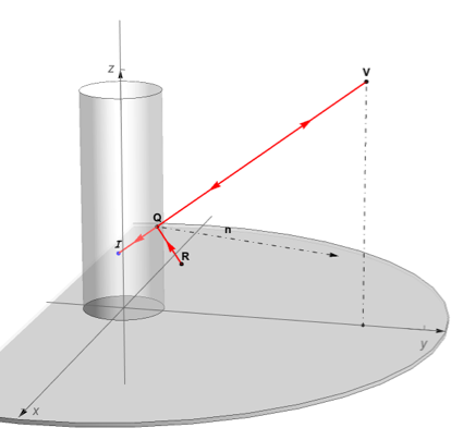
The viewer at V perceives the anamorphic points R as points I, the artist has to create anamorphic points R from the reflected points I. Based on three observations, a function (anamorphCyl3D) can be made that maps the reflected image points [ScriptCapitalI] into their anamorphic match R:
- both I and R are in the same horizontal plane: zi=zr
- the lines VQ and RQ form equal angles with the normal n at Q according to the law of reflection
the distances IQ and RQ are equal per the same law of reflection
anamorphCyl3D[(*image point position*)
  iPt : {xi_, yi_, zi_},(*viewpoint*)vPt : {0, yv_, zv_}] :=

 Quiet@Module[{t, R1, R2, hi = 5, qPt, nV, aV, rV, vV, solt},
   (*view line*)R1 = InfiniteLine[{iPt, vPt}];
   (*cylinder hull: mirror*)
   R2 = RegionBoundary[Cylinder[{{0., 0, 0}, {0, 0, 10}}, 1.]];
   (*intersection point nearest to viewpoint*)
   qPt = Nearest[{x, y, z} /.
       NSolve[{x, y, z} \[Element] R1 && {x, y, z} \[Element] R2, {x,
         y, z}, Reals], vPt][[1]];
   (*view vector*)vV = vPt - iPt;
   (*normal vector at qPt*)nV = {qPt[[1]], qPt[[2]], 0};
   (*vertical dropdown from vPt*)aV = Projection[vV, nV] - vV;
   (*reflection vector of vPt from iPt*)rV = vV + 2 aV;
   t = -(qPt[[3]] - iPt[[3]])/rV[[3]];
   (*anamorphic point*)t rV + qPt]
This function can be simplified and compiled to increase the speed. This is more than necessary since we will have to process hundreds, if not thousands of points:
anamorphCyl3DCF =
 Compile[{{xi, _Real}, {yi, _Real}, {zi, _Real}, {yv, _Real}},
  Module[{t1, t2},
   t1 = Sqrt[(yi - yv)^2 - xi^2 (-1 + yv^2)];
   t2 = 1/(xi^2 + (yi -
         yv)^2); {-t2^2 xi ((xi^2 + (yi - yv)^2) ((yi - yv) yv +
          t1) - (xi^2 + yi^2 - yi yv +
          t1) (xi^2 (-1 + 2 yv^2) - (yi - yv) (yi - yv + 2 yv t1))),
    t2 (xi^2 yv + (-yi + yv) t1 +
       t2 (xi^2 + yi^2 - yi yv + t1) (-(yi - yv)^3 +
          xi^2 (-yi + yv + 2 yi yv^2 - 2 yv^3 + 2 yv t1))), zi}],
  CompilationTarget -> "C", Parallelization -> True,
  RuntimeOptions -> "Speed"]
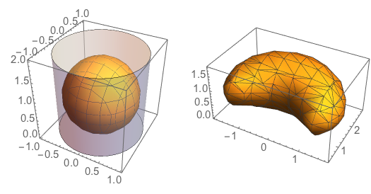
Let's try this first by applying the function to points on the surface of an object defined by ListSurfacePlot, e.g a sphere:
sphere =(*points on the spere surface*)
  Flatten[Table[.9 {Cos[\[Phi]] Sin[\[Theta]],
      Sin[\[Phi]] Sin[\[Theta]], 1. - Cos[\[Theta]]}, {\[Phi], 0.,
     2 \[Pi], \[Pi]/16}, {\[Theta], 0., \[Pi], \[Pi]/16}], 1];
anamorphicSphere =(*their anamorphic counterpart*)

  Map[anamorphCyl3DCF @@ Flatten[{#, 6.}] &, sphere];
GraphicsRow[{Graphics3D[{{Opacity[.35],
     Cylinder[{{0, 0, 0}, {0, 0, 2}}, 1]},
    ListSurfacePlot3D[sphere, Mesh -> All][[1]]}, Axes -> True],
  ListSurfacePlot3D[anamorphicSphere, Mesh -> All,
   PerformanceGoal -> "Quality", PlotTheme -> "ThickSurface"]},
 ImageSize -> 350]
Or we could apply the function directly inside a ParametricPlot3D object, e.g. a torus
GraphicsRow[{ParametricPlot3D[.33 {(2 + Cos[v]) Cos[u], Sin[v],
     3. + (2 + Cos[v]) Sin[u]}, {u, 0, 2. \[Pi]}, {v, 0, 2. \[Pi]}],
  ParametricPlot3D[ anamorphCyl3DCF @@ Flatten[{#, 6.}] &[.33 {(2 + Cos[v]) Cos[u],
      Sin[v], 3. + (2 + Cos[v]) Sin[u]}], {u, 0, 2. \[Pi]}, {v, 0, 2. \[Pi]}]}, ImageSize -> 350]
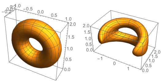
Here we see both the reflected torus and its anamorphic counterpart together with the cylindric mirror. One can rotate the torus along one of its main axes or change the distance of the observer's eye from the center of the mirror.
Manipulate[
 Module[{torus},
  torus = RotationMatrix[\[Theta],
     Switch[dir, 1, {1, 0, 0},
      2, {0, 0, 1}]].   (.33 {Cos[u] (2 + Cos[v]),
       Sin[v], (2 + Cos[v]) Sin[u]});
  Quiet@Show[{
     ParametricPlot3D[torus, {u, 0, 2. \[Pi]}, {v, 0, 2. \[Pi]},
      Mesh -> 10, PlotPoints -> 25],
     ParametricPlot3D[
      anamorphCyl3DCF @@ Flatten[{#, yv}] &[torus], {u, 0,
       2. \[Pi]}, {v, 0, 2. \[Pi]}, Mesh -> 10, PlotPoints -> 36],
     Graphics3D[{Cylinder[{{0, 0, -1}, {0, 0, -.99}}, 5],
       Opacity[.35], Cylinder[{{0, 0, -1}, {0, 0, 2}}, 1]}]},
    PlotRange -> {{-2, 2}, {-1, 3.5}, {-1, 2}}, Axes -> False,
    Boxed -> False, ViewPoint -> {0, 2., 3.1}, ImageSize -> 250]],
 "eye distance", {{yv, 6., ""}, 2, 24, ImageSize -> Small},
 "\nrotation angle", {{\[Theta], 0., ""}, -\[Pi], \[Pi],
  ImageSize -> Small},
 Row[{"\nrotation axis",
   Control[{{dir, 1, ""}, {1 -> "x-axis", 2 -> "z-axis"}}]}],
 ControlPlacement -> Left, SynchronousUpdating -> True]
We can now also apply this function to the vertices of a polygonal mesh of a discretized object. For example, the ones from ExampleDtata, "Geometry3D" in the Wolfram Language [1]. We first need to scale the coordinates within the limits of a right cylinder with radius 1, centered around the z-axis:
getAndRescale[example_String] :=
 Module[{data, ranges, maxRange, temp1, temp2},
  data = ExampleData[{"Geometry3D", example}, "PolygonObjects"];
  ranges = MinMax@Flatten[data[[All, 1]], 1][[All, #]] & /@ Range[3];
  maxRange = MaximalBy[Most@ranges, Abs[Subtract @@ #] &];
  temp1 = MapAt[Rescale[#, First@maxRange, {-1., 1.}] &,
    data, {All, 1, All, 1}];
  MapAt[Rescale[#,
     Last@ranges, {0,
      2*Subtract @@ ranges[[3]]/Subtract @@ ranges[[1]]}] &,
   temp1, {All, 1, All, 3}]]
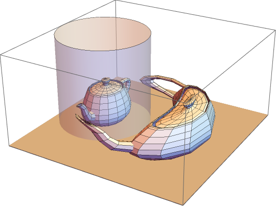
Applied to the "UtahTeapot":
Module[{yv = 6., data, anaData},
 data = getAndRescale["UtahTeapot"];
 anaData = Map[anamorphCyl3DCF @@ Flatten[{.96 #, yv}] &, data, {3}];
 g = Graphics3D[anaData];
 Graphics3D[{data,
   anaData, {LightGray,
    Cylinder[{{0, 0, 0}, {0, 0, .01}}, 10]}, {Opacity[.35],
    Cylinder[{{0, 0, 0}, {0, 0, 2}}, 1]}},
  PlotRange -> {{-2, 2}, {-1, 3}, {0, 2}},
  ViewPoint -> {2.65, 1.6, 1.45}]]
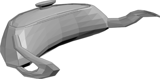
The anamorphic teapot can now be printed using Printout3D and uploaded to an online 3D printing service as e.g. 3DHubs:
Printout3D[g, "3DHubs", RegionSize -> Quantity[8, "Centimeters"]]
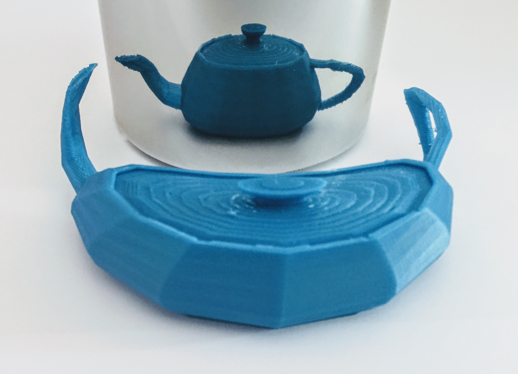
Afterwards, this can be tested in the reflection of a real homemade cylindrical mirror [2]:
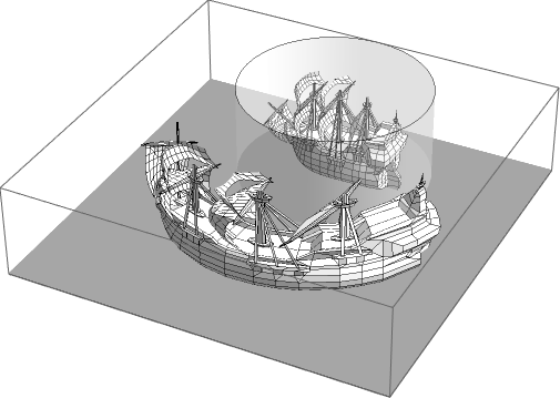
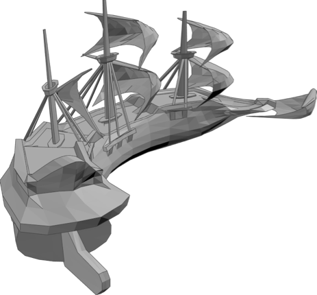
Or we can try the "Galleon" saved as an STL file with Printout3D:
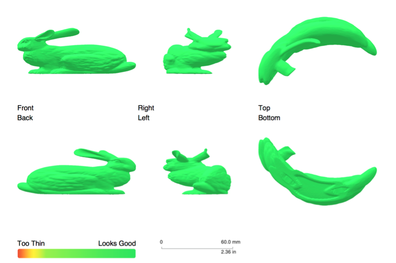
And we could try the famous Stanford Bunny with almost 70k polygons uploaded with Printout3D to 3D printer Sculpteo:
Any more artists out there that want to try their skills at 3D anamorphic printing using Mathematica?
Remarks
[1] By mapping the vertices of polygonal meshes to their anamorphic counterpart and drawing a straight line between the vertices, we get the same limitation a with the original: only an infinite number of vertices will give the absolute correct object. But this is hardly a limitation to get an interesting result...
[2] Cardboard cylinder from a discarded salt dispenser. Reflective window film glued around it. Diameter 60mm.


