Story Time
At its first meeting in 1922, the International Astronomical Union (IAU), officially adopted the list of 88 constellations that we use today. These include 14 men and women, 9 birds, two insects, 19 land animals, 10 water creatures, two centaurs, one head of hair, a serpent, a dragon, a flying horse, a river and 29 inanimate objects. As many of us have (frustratingly) witnessed first hand while star-gazing - most of these bear little resemblance to their supposed figures. Instead, it is more likely that the ancient constellation-makers meant them to be symbolic, a kind of celestial "Hall of Fame" for their favorite animals or heroes.
This begs two questions I sought to answer with this project:
- Can we 'do better' now with the WL's StarData[] curated data and Machine Learning functionality?
- What if the ancient constellation-makers were slightly more creative? Say they looked up at the sky, and only saw yoga-poses!
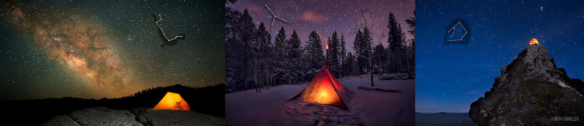
Some examples of the found yoga-pose constellations, projected on images of the night sky are shown here, with a walk-through of the code below:
Yoga Poses
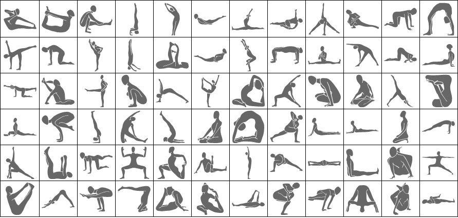
First things first, finding images for yoga poses. Turns out, the WL has a built in YogaPose Entity Class with 216(!) available entities and their schematics. A lot of these are very similar (e.g. palms facing up/down) and we therefore only select a subset of them, which differ substantially from each other:
yogaposes = EntityClass["YogaPose", All] // EntityList;
chosenPoses =
  List /@ {4, 6, 7, 8, 11, 14, 23, 25, 28, 35, 38, 43, 51, 54, 56, 59,
     63, 65, 71, 72, 76, 77, 78, 84, 88, 90, 98, 100, 102, 103, 110,
    111, 112, 113, 116, 118, 119, 125, 126, 133, 139, 142, 149, 152,
    153, 154, 155, 156, 160, 164, 165, 167, 172, 177, 178, 180, 182,
    183, 184, 190, 193, 194, 195, 197, 202, 204, 206, 207, 209, 210,
    212, 215, 216};
Shallow[Extract[yogaposes, chosenPoses]]
We write a wrapper to ensure the schematics are padded to give a square image and visualize our 73 constellations:
makeSquare[gr_, size_, bool_: False] :=
 Block[{range, magnitudes, order, padding, newRanges, res},
  range = AbsoluteOptions[gr, PlotRange][[1, 2]];
  magnitudes = Abs[Subtract @@@ range];
  order = Ordering[magnitudes, 2, Greater];
  padding = Subtract @@ magnitudes[[order]]/2;
  newRanges = {{-1, 1} padding + Last[range[[order]]],
    First[range[[order]]]};
  res = Show[gr, PlotRange -> Reverse@newRanges[[order]],
    ImageSize -> size];
  If[bool, Rasterize[res], res]]

Multicolumn[
 makeSquare[#["SimplifiedSchematic"], 64] & /@
  Most[Extract[yogaposes, chosenPoses]], 9, Frame -> All]
Neural Network
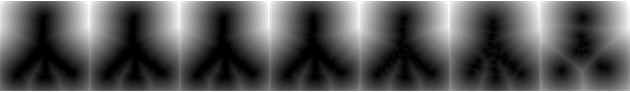
Our problem now can be worded as a classification one: given 5-10 stars, classify them as one of the 73 yoga-poses constellations The problem with that formulation of-course is that 5-10 randomly selected points inside the constellation region isn't specific enough to differentiate between constellations. The image below shows that although 1000 sets of 10 points will define the shape, 10 points alone fall short:
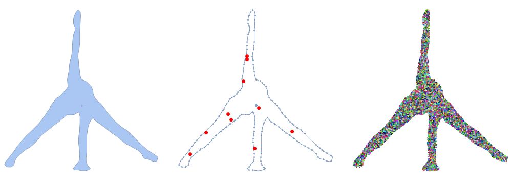
Instead, we compute the Voronoi diagram of the points, using DistanceTransform to leverage already-optimized convolutional neural nets used for classifying images. Note that, even if (naturally) the results are less clear with fewer points (left to right) - the result with only 10 points at the far right is still quite recognizable to a human eye:
With this in-mind, we create a neural network similar to the VGG16 neural network, with successive 5x5 convolutions, ReLu activation functions and Max pooling layers. Finally note that we use an average pooling instead of fully connected layers to reduce the number of parameters and the use of dropout layers.
conv[output_] := ConvolutionLayer[output, {5, 5}, "PaddingSize" -> 2]
pool[size_] := PoolingLayer[{size, size}, "Stride" -> size]
lenet = NetChain[
  {conv[32], Ramp, conv[32], Ramp, pool[2], conv[64], Ramp, conv[64],
   Ramp, pool[2], conv[128], Ramp, conv[128], Ramp, conv[128], Ramp,
   PoolingLayer[{9, 9}, "Stride" -> 9, "Function" -> Mean],
   FlattenLayer[], DropoutLayer[], 73, SoftmaxLayer[]},
  "Output" -> NetDecoder[{"Class", Extract[yogaposes, chosenPoses]}],
  "Input" -> NetEncoder[{"Image", {64, 64}, ColorSpace -> "Grayscale"}]
  ]
The training set then consists of generating 10-15 points inside the constellation region (resized and padded to allow for rotations later), and taking their DistanceTransform:
meshes[n_] :=
 meshes[n] =
  ImagePad[ColorNegate@
    makeSquare[
     yogaposes[[chosenPoses[[n, 1]]]]["SimplifiedSchematic"], 44], 10]
trainingSet[n_, m_, iter_] :=
 With[{reg =
    ImageMesh[meshes[n], CornerNeighbors -> False,
     Method -> "MarchingSquares"]},
  Thread[ColorConvert[
       ImageAdjust[
        DistanceTransform[Image[SparseArray[# -> 0, {64, 64}, 1]]]],
       "Grayscale"] & /@
     Clip[Round@RandomPoint[reg, {iter, m}], {1, 64}] ->
    yogaposes[[chosenPoses[[n, 1]]]]]]
exampleTrainingSet =
 Flatten[trainingSet[#, 10, 1] & /@ RandomInteger[{1, 73}, 10], 1]
The net took a couple of hours to train on ~100,000 examples on my CPU. Here we import the trained net:
lenetTrained = Import["constellationsNet.wlnet"]
Night Sky
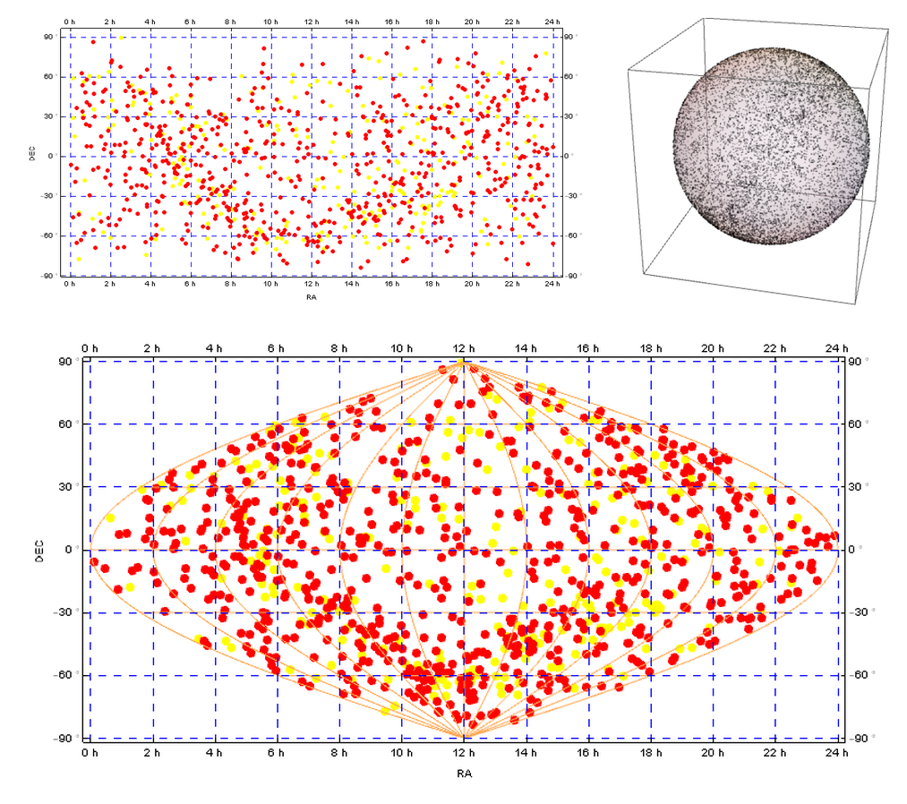
We're almost ready to classify the night sky. We first need the location of the 10,000 brightest stars along with their Right Ascension and Declination:
brightest =
 StarData[EntityClass[
   "Star", {EntityProperty["Star", "ApparentMagnitude"] ->
     TakeSmallest[10000]}], {"RightAscension", "Declination",
   "ApparentMagnitude"}]
We can plot these on the night sky using no projection (i.e. RA Vs Dec), using the sinusoidal projection (taken by Kuba's excellent answer in SE) or on the celestial sphere given by the following transformations respectively:
$$sinusoidal:\{(\alpha -\pi ) \cos (\delta ),\delta \}$$
$$map to3D:\{\cos (\alpha ) \cos (\delta ),\sin (\alpha ) \cos (\delta ),\sin (\delta )\}$$
Classification
Finally, we use these 10,000 brightest stars to compute a multivariate smooth kernel distribution out of which to sample from and a Nearest function to compute neighboring stars. We need to of-course use our own distance function on the celestial sphere:
wrap[list_] := Block[{xs, ys},
  {xs, ys} = Transpose[list];
  Thread[{Mod[xs, 2 \[Pi]], Mod[ys, \[Pi], -\[Pi]/2]}]]
mapTo3D[\[Alpha]_, \[Delta]_] = {Cos[\[Alpha]] Cos[\[Delta]],
   Cos[\[Delta]] Sin[\[Alpha]], Sin[\[Delta]]};
dist[{u_, v_}, {x_,
   y_}] := (#1[[1]] - #2[[1]])^2 + (#1[[2]] - #2[[2]])^2 + (#1[[
       3]] - #2[[3]])^2 & @@ mapTo3D @@@ {{u, v}, {x, y}}
pts = wrap@QuantityMagnitude[UnitConvert[brightest[[6 ;;, ;; 2]]]];
nf = Nearest[pts, DistanceFunction -> dist]
sm = SmoothKernelDistribution[pts]
Our search algorithm is therefore defined as follows:
- Pick a random position from the night sky distribution
- Compute its 5-10 nearest neighbors
- Classify those stars and their rotations by $\frac{2 \pi }{15}$
- Select the rotation which gives the highest accuracy
Associate constellation to running association and repeat
rescale[list_] := Block[{xs, ys},
  {xs, ys} = Thread[list];
  Thread[Rescale[#, MinMax[#], {11, 54}] & /@ {xs, ys}]]
rotate[\[Alpha]_, pts_] :=
 ImageAdjust@
  DistanceTransform[
   Image@SparseArray[
     Round@RotationTransform[\[Alpha] , {65/2, 65/2}][rescale[pts]] ->
       0, {64, 64}, 1]]
sky = <||>;
accumulate[] :=
 Block[{pts =
    nf[Mod[RandomVariate[sm] + {0, \[Pi]}, 2 \[Pi]] - {0, \[Pi]},
     RandomInteger[{5, 10}]], \[Alpha], pred},
  {\[Alpha], pred} =
   Last[SortBy[
     First /@
      Table[Thread[{\[Alpha],
         lenetTrained[rotate[\[Alpha], pts],
          "TopProbabilities"]}], {\[Alpha], 0, 2 \[Pi], (2 \[Pi])/
        15}], Last]];
  If[Not[KeyExistsQ[sky, pred[[1]]]] ||
    TrueQ[sky[pred[[1]], "Accuracy"] < pred[[2]]],
   AssociateTo[sky,
    pred[[1]] -> <|"Accuracy" -> pred[[2]],
      "Image" ->
       HighlightImage[
        makeSquare[pred[[1]]["SimplifiedSchematic"],
         64], {PointSize[Medium], Red,
         Round[RotationTransform[\[Alpha], 65/2 {1, 1}][rescale@pts],
          0.5]}], "Points" -> pts, "Angle" -> \[Alpha]|>], Nothing];]
We can import a precomputed association with 20 such constellations:
selectedAsc = Import["skyAsc.m.gz"]
Results
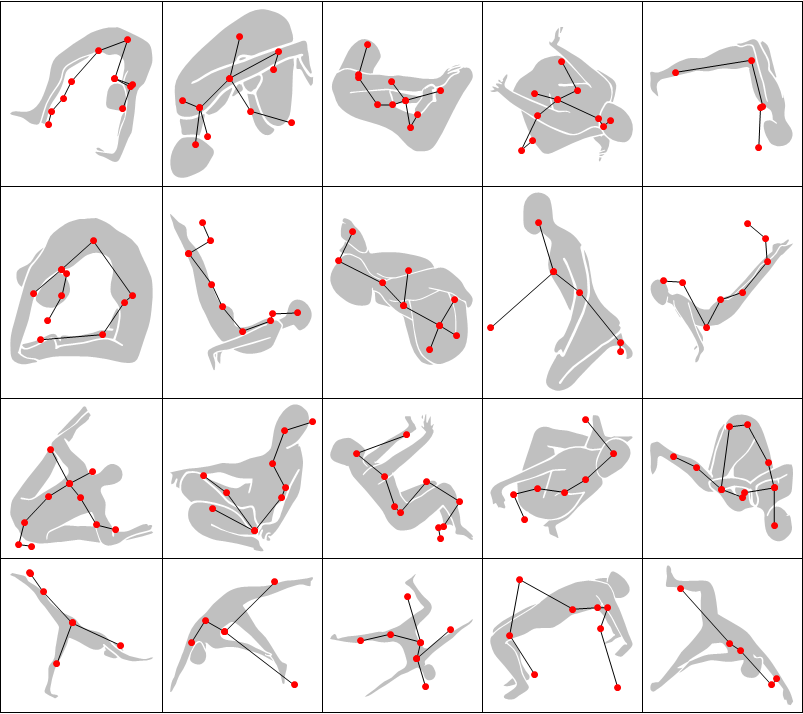
Finally, we orient the schematic based on the optimally found angle and (manually) connect the dots.
orient[pts_, \[Alpha]_] :=
 Round[RotationTransform[\[Alpha], 65/2 {1, 1}][rescale@pts], 0.5]
lines = {{{10, 7, 3, 1, 4, 9, 2, 5, 8}, {2, 6}}, {{7, 3, 1, 9,
     6}, {10, 2, 1, 8}, {4, 3, 5}}, {{7, 8, 9, 4, 3, 2, 10}, {1, 2, 6,
      5}}, {{10, 2, 1, 3, 9, 5}, {7, 1, 4, 6, 8}}, {{5, 4, 1, 2,
     3}}, {{10, 4, 5, 7, 9, 3, 8}, {6, 1, 2, 3}}, {{9, 5, 6, 3, 1, 2,
     7}, {7, 4, 8}}, {{7, 6, 2, 3, 5, 8}, {9, 5, 4}, {3, 1}}, {{6, 2,
     1, 3, 4}, {2, 5}}, {{5, 6, 4, 1, 2, 8, 3, 7}}, {{10, 6, 3, 2,
     7}, {5, 2, 1, 4, 9, 8}}, {{9, 5, 1, 2, 4, 8, 7}, {6, 3, 8}}, {{6,
      10, 4, 2, 1, 3, 9, 7, 5, 8}}, {{6, 7, 3, 2, 1, 4, 5}}, {{10, 8,
     3, 6, 7, 2, 5, 9}, {5, 1, 4, 3}}, {{6, 5, 2, 1, 3}, {1, 4}}, {{5,
      1, 2, 3}, {1, 4}}, {{6, 3, 2, 1, 4}, {3, 5}, {2, 7}}, {{3, 6, 8,
      2, 4, 5, 1, 7}}, {{3, 1, 2, 6, 5}}};
makeSquareAndScale[gr_, \[Alpha]_, size_, opacity_] :=
 Block[{range, magnitudes, order, padding, newRanges, s},
  range = AbsoluteOptions[gr, PlotRange][[1, 2]];
  magnitudes = Abs[Subtract @@@ range];
  order = Ordering[magnitudes, 2, Greater];
  padding = Subtract @@ magnitudes[[order]]/2;
  s = size/First[magnitudes[[order]]];
  newRanges = {{-1, 1} padding + Last[range[[order]]],
    First[range[[order]]]};
  Graphics[{Opacity[opacity],
    GeometricTransformation[
     GeometricTransformation[
      gr[[1]], {ScalingMatrix[{s,
         s}], -1 First /@ (s Reverse@newRanges[[order]])}],
     RotationTransform[\[Alpha], (size + 1)/2 {1, 1}]]},
   ImageSize -> size]]
With[{l = Map[Line, lines, {2}]},
 Multicolumn[
  Table[Show[
    makeSquareAndScale[
     Keys[selectedAsc][[i]][
      "SimplifiedSchematic"], -selectedAsc[[i, -1]], 64, 0.25],
    Graphics[
     GraphicsComplex[
      rescale[selectedAsc[[i, -2]]], {l[[i]], Red, PointSize[Large],
       Point /@ Sort /@ Flatten /@ lines[[i]]}]],
    ImageSize -> 150], {i, 20}], 5, Frame -> All,
  Appearance -> "Horizontal"]]
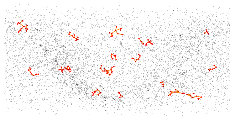
These can also be superimposed on the full night-sky:
Graphics[{With[{l = Map[Line, lines, {2}]},
   Table[GraphicsComplex[
     selectedAsc[[i, -2]], {Orange, Thickness[Large], l[[i]], Red,
      PointSize[Medium], Point /@ Sort /@ Flatten /@ lines[[i]]}], {i,
      20}]], Opacity[0.25], PointSize[Small],
  Point[Complement[pts, Flatten[Values@selectedAsc[[All, -2]], 1]]]},
 ImageSize -> 750]
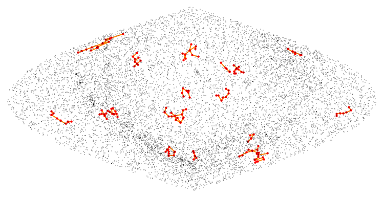
sinusoidal[\[Alpha]_, \[Delta]_] = {(\[Alpha] - \[Pi]) Cos[\[Delta]], \
\[Delta]}
Graphics[{With[{l = Map[Line, lines, {2}]},
   Table[GraphicsComplex[
     sinusoidal @@@ selectedAsc[[i, -2]], {Orange, Thickness[Large],
      l[[i]], Red, PointSize[Medium],
      Point /@ Sort /@ Flatten /@ lines[[i]]}], {i, 20}]],
  Opacity[0.25], PointSize[Small],
  Point[sinusoidal @@@
    Complement[pts, Flatten[Values@selectedAsc[[All, -2]], 1]]]},
 ImageSize -> 750]
It is then a matter of Overlaying these found constellations to existing images of night skies to produce the images at the beginning of the post:
overlay[{img_, constellation_}, {size_, loc_, opac_}] :=
 ImageCompose[imgs[[img]],
  ImageResize[
   Show[makeSquareAndScale[
     Keys[selectedAsc][[constellation]][
      "SimplifiedSchematic"], -selectedAsc[[constellation, -1]], 64,
     opac], Graphics[
     GraphicsComplex[
      rescale[selectedAsc[[constellation, -2]]], {White,
       Thickness[0.0075], Line /@ lines[[constellation]], White,
       PointSize[.025],
       Point /@ Sort /@ Flatten /@ lines[[constellation]]}]],
    ImageSize -> 1000], size], Scaled[loc]]
Conclusions / Lessons Learned
- It IS possible to find collections of stars in the night sky matching all sorts of shapes. Other built-in entities to try are Pokemons, Dinosaurs etc
- Not all the found constellation work 'perfectly'
- Machine Learning is a powerful tool, and the WL implementation makes it easy to get started
- Reformulating the problem to an easier, already solved problem (e.g. points -> 2D image input) can help Classification Accuracy
- Perhaps the most interesting aspect of neural networks now, is diversifying its applications - so be creative
This work was presented at the 2017 WTC (as part of a larger talk entitled "(De)Generative Art").
I look forward to any comments/suggestions.
George
PS The editor doesn't seem to let me attach the .wlnet and .m.gz files.


