Message Boards Message Boards

Solver for unsteady flow with the use of Mathematica FEM

fig7

I started the discussion here but I also want to repeat on this forum. There are many commercial and open code for solving the problems of unsteady flows. We are interested in the possibility of solving these problems using Mathematica FEM. Previously proposed solvers for stationary incompressible isothermal flows:

Solving 2D Incompressible Flows using Finite Elements: http://community.wolfram.com/groups/-/m/t/610335

FEM Solver for Navier-Stokes equations in 2D: http://community.wolfram.com/groups/-/m/t/611304

Nonlinear FEM Solver for Navier-Stokes equations in 2D: https://mathematica.stackexchange.com/questions/94914/nonlinear-fem-solver-for-navier-stokes-equations-in-2d/96579#96579

We give several examples of the successful application of the finite element method for solving unsteady problem including nonisothermal and compressible flows. We will begin with two standard tests that were proposed to solve this class of problems by

M. Schäfer and S. Turek, Benchmark computations of laminar ?ow around a cylinder (With support by F. Durst, E. Krause and R. Rannacher). In E. Hirschel, editor, Flow Simulation with High-Performance Computers II. DFG priority research program results 1993-1995, number 52 in Notes Numer. Fluid Mech., pp.547–566. Vieweg, Weisbaden, 1996. https://www.uio.no/studier/emner/matnat/math/MEK4300/v14/undervisningsmateriale/schaeferturek1996.pdf

fig8

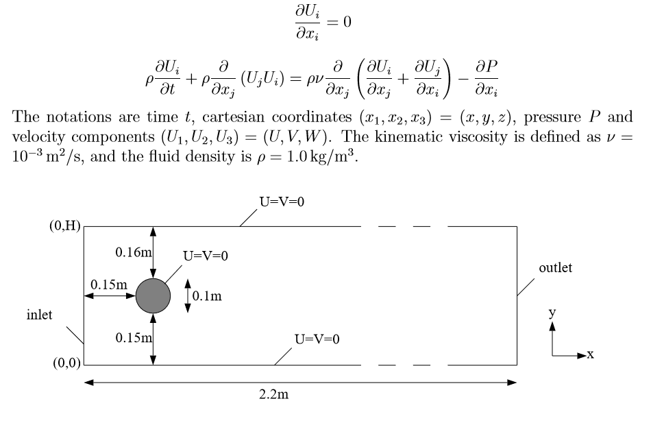
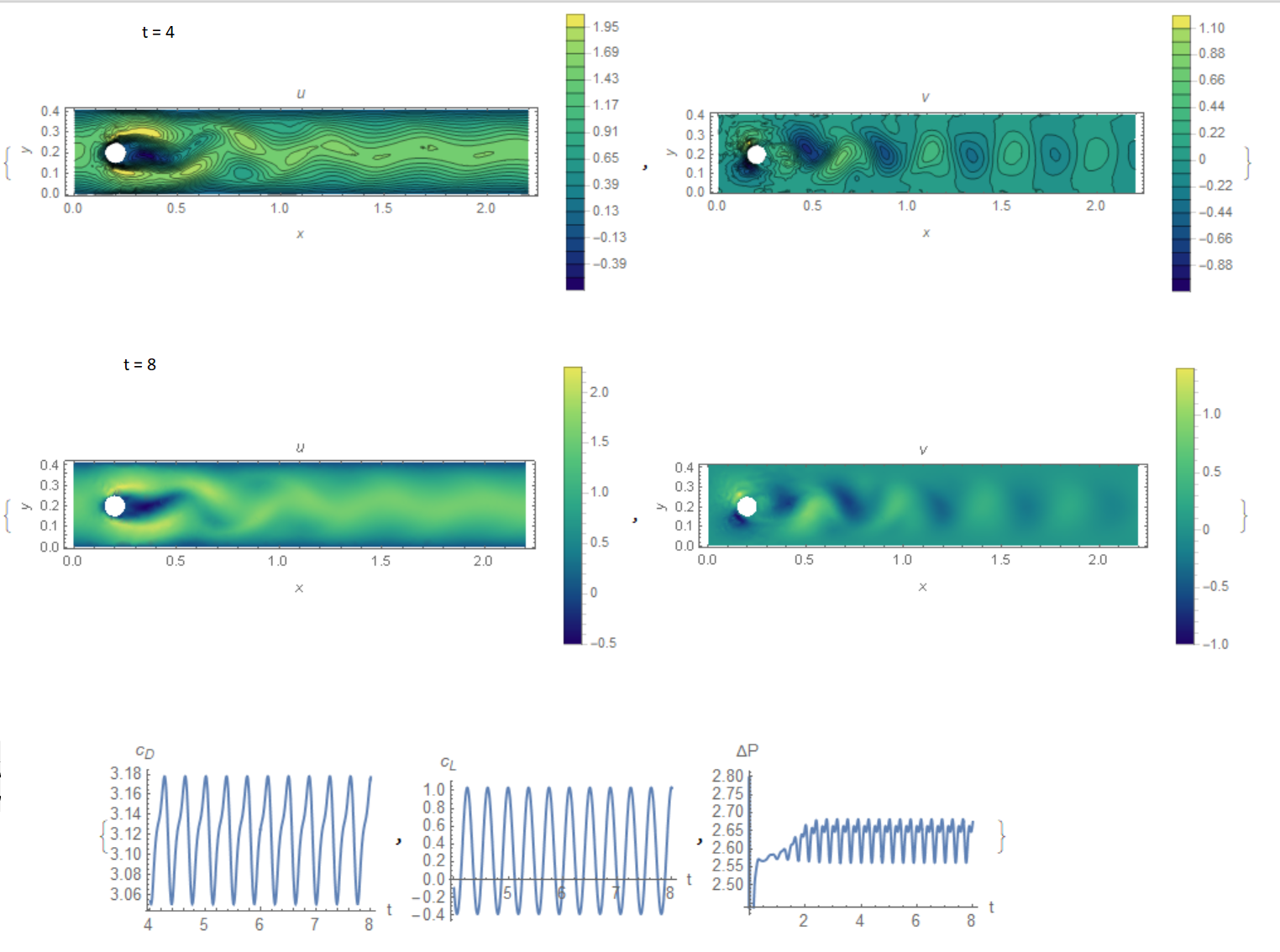
Let us consider the flow in a flat channel around a cylinder at Reynolds number = 100, when self-oscillations occur leading to the detachment of vortices in the aft part of cylinder. In this problem it is necessary to calculate drag coe?cient, lift coe?cient and pressure di?erence in the frontal and aft part of the cylinder as functions of time, maximum drag coe?cient, maximum lift coe?cient , Strouhal number and pressure di?erence $\Delta P(t)$ at $t = t0 +1/2f$. The frequency f is determined by the period of oscillations of lift coe?cient f=f(c_L). The data for this test, the code and the results are shown below.

H = .41; L = 2.2; {x0, y0, r0} = {1/5, 1/5, 1/20}; 
? = RegionDifference[Rectangle[{0, 0}, {L, H}], Disk[{x0, y0}, r0]];
RegionPlot[?, AspectRatio -> Automatic]

K = 2000; Um = 1.5; ? = 10^-3; t0 = .004;
U0[y_, t_] := 4*Um*y/H*(1 - y/H)
UX[0][x_, y_] := 0;
VY[0][x_, y_] := 0;
P0[0][x_, y_] := 0;
Do[
  {UX[i], VY[i], P0[i]} = 
   NDSolveValue[{{Inactive[
           Div][({{-?, 0}, {0, -?}}.Inactive[Grad][
             u[x, y], {x, y}]), {x, y}] + 
\!\(\*SuperscriptBox[\(p\), 
TagBox[
RowBox[{"(", 
RowBox[{"1", ",", "0"}], ")"}],
Derivative],
MultilineFunction->None]\)[x, y] + (u[x, y] - UX[i - 1][x, y])/t0 + 
         UX[i - 1][x, y]*D[u[x, y], x] + 
         VY[i - 1][x, y]*D[u[x, y], y], 
        Inactive[
           Div][({{-?, 0}, {0, -?}}.Inactive[Grad][
             v[x, y], {x, y}]), {x, y}] + 
\!\(\*SuperscriptBox[\(p\), 
TagBox[
RowBox[{"(", 
RowBox[{"0", ",", "1"}], ")"}],
Derivative],
MultilineFunction->None]\)[x, y] + (v[x, y] - VY[i - 1][x, y])/t0 + 
         UX[i - 1][x, y]*D[v[x, y], x] + 
         VY[i - 1][x, y]*D[v[x, y], y], 
\!\(\*SuperscriptBox[\(u\), 
TagBox[
RowBox[{"(", 
RowBox[{"1", ",", "0"}], ")"}],
Derivative],
MultilineFunction->None]\)[x, y] + 
\!\(\*SuperscriptBox[\(v\), 
TagBox[
RowBox[{"(", 
RowBox[{"0", ",", "1"}], ")"}],
Derivative],
MultilineFunction->None]\)[x, y]} == {0, 0, 0} /. ? -> ?, {
      DirichletCondition[{u[x, y] == U0[y, i*t0], v[x, y] == 0}, 
       x == 0.], 
      DirichletCondition[{u[x, y] == 0., v[x, y] == 0.}, 
       0 <= x <= L && y == 0 || y == H], 
      DirichletCondition[{u[x, y] == 0, 
        v[x, y] == 0}, (x - x0)^2 + (y - y0)^2 == r0^2], 
      DirichletCondition[p[x, y] == P0[i - 1][x, y], x == L]}}, {u, v,
      p}, {x, y} ? ?, 
    Method -> {"FiniteElement", 
      "InterpolationOrder" -> {u -> 2, v -> 2, p -> 1}, 
      "MeshOptions" -> {"MaxCellMeasure" -> 0.001}}], {i, 1, K}];
{ContourPlot[UX[K/2][x, y], {x, y} ? ?, 
   AspectRatio -> Automatic, ColorFunction -> "BlueGreenYellow", 
   FrameLabel -> {x, y}, PlotLegends -> Automatic, Contours -> 20, 
   PlotPoints -> 25, PlotLabel -> u, MaxRecursion -> 2], 
  ContourPlot[VY[K/2][x, y], {x, y} ? ?, 
   AspectRatio -> Automatic, ColorFunction -> "BlueGreenYellow", 
   FrameLabel -> {x, y}, PlotLegends -> Automatic, Contours -> 20, 
   PlotPoints -> 25, PlotLabel -> v, MaxRecursion -> 2, 
   PlotRange -> All]} // Quiet
{DensityPlot[UX[K][x, y], {x, y} ? ?, 
   AspectRatio -> Automatic, ColorFunction -> "BlueGreenYellow", 
   FrameLabel -> {x, y}, PlotLegends -> Automatic, PlotPoints -> 25, 
   PlotLabel -> u, MaxRecursion -> 2], 
  DensityPlot[VY[K][x, y], {x, y} ? ?, 
   AspectRatio -> Automatic, ColorFunction -> "BlueGreenYellow", 
   FrameLabel -> {x, y}, PlotLegends -> Automatic, PlotPoints -> 25, 
   PlotLabel -> v, MaxRecursion -> 2, PlotRange -> All]} // Quiet
dPl = Interpolation[
   Table[{i*t0, (P0[i][.15, .2] - P0[i][.25, .2])}, {i, 0, K, 1}]];


cD = Table[{t0*i, NIntegrate[(-?*(-Sin[?] (Sin[?] 
\!\(\*SuperscriptBox[\(UX[i]\), 
TagBox[
RowBox[{"(", 
RowBox[{"0", ",", "1"}], ")"}],
Derivative],
MultilineFunction->None]\)[x0 + r Cos[?], 
                 y0 + r Sin[?]] + Cos[?] 
\!\(\*SuperscriptBox[\(UX[i]\), 
TagBox[
RowBox[{"(", 
RowBox[{"1", ",", "0"}], ")"}],
Derivative],
MultilineFunction->None]\)[x0 + r Cos[?], 
                 y0 + r Sin[?]]) + Cos[?] (Sin[?] 
\!\(\*SuperscriptBox[\(VY[i]\), 
TagBox[
RowBox[{"(", 
RowBox[{"0", ",", "1"}], ")"}],
Derivative],
MultilineFunction->None]\)[x0 + r Cos[?], 
                 y0 + r Sin[?]] + Cos[?] 
\!\(\*SuperscriptBox[\(VY[i]\), 
TagBox[
RowBox[{"(", 
RowBox[{"1", ",", "0"}], ")"}],
Derivative],
MultilineFunction->None]\)[x0 + r Cos[?], 
                 y0 + r Sin[?]]))*Sin[?] - 
         P0[i][x0 + r Cos[?], y0 + r Sin[?]]*
          Cos[?]) /. {r -> r0}, {?, 0, 2*Pi}]}, {i, 
     1000, 2000}]; // Quiet

cL = Table[{t0*i, -NIntegrate[(-?*(-Sin[?] (Sin[?] 
\!\(\*SuperscriptBox[\(UX[i]\), 
TagBox[
RowBox[{"(", 
RowBox[{"0", ",", "1"}], ")"}],
Derivative],
MultilineFunction->None]\)[x0 + r Cos[?], 
                  y0 + r Sin[?]] + Cos[?] 
\!\(\*SuperscriptBox[\(UX[i]\), 
TagBox[
RowBox[{"(", 
RowBox[{"1", ",", "0"}], ")"}],
Derivative],
MultilineFunction->None]\)[x0 + r Cos[?], 
                  y0 + r Sin[?]]) + 
             Cos[?] (Sin[?] 
\!\(\*SuperscriptBox[\(VY[i]\), 
TagBox[
RowBox[{"(", 
RowBox[{"0", ",", "1"}], ")"}],
Derivative],
MultilineFunction->None]\)[x0 + r Cos[?], 
                  y0 + r Sin[?]] + Cos[?] 
\!\(\*SuperscriptBox[\(VY[i]\), 
TagBox[
RowBox[{"(", 
RowBox[{"1", ",", "0"}], ")"}],
Derivative],
MultilineFunction->None]\)[x0 + r Cos[?], 
                  y0 + r Sin[?]]))*Cos[?] + 
          P0[i][x0 + r Cos[?], y0 + r Sin[?]]*
           Sin[?]) /. {r -> r0}, {?, 0, 2*Pi}]}, {i, 
     1000, 2000}]; // Quiet
{ListLinePlot[cD, 
  AxesLabel -> {"t", "\!\(\*SubscriptBox[\(c\), \(D\)]\)"}], 
 ListLinePlot[cL, 
  AxesLabel -> {"t", "\!\(\*SubscriptBox[\(c\), \(L\)]\)"}], 
 Plot[dPl[x], {x, 0, 8}, AxesLabel -> {"t", "?P"}]}

f002 = FindFit[cL, a*.5 + b*.8*Sin[k*16*t + c*1.], {a, b, k, c}, t]


Plot[Evaluate[a*.5 + b*.8*Sin[k*16*t + c*1.] /. f002], {t, 4, 8}, 
 Epilog -> Map[Point, cL]]

k0=k/.f002;
Struhalnumber = .1*16*k0/2/Pi


cLm = MaximalBy[cL, Last]

sol = {Max[cD[[All, 2]]], Max[cL[[All, 2]]], Struhalnumber, 
  dPl[cLm[[1, 1]] + Pi/(16*k0)]}

In Fig. 1 shows the components of the flow velocity and the required coefficients. Our solution of the problem and what is required in the test

{3.17805, 1.03297, 0.266606, 2.60427}

lowerbound= { 3.2200, 0.9900, 0.2950, 2.4600};
upperbound = {3.2400, 1.0100, 0.3050, 2.5000};

Fig1 Note that our results differ from allowable by several percent, but if you look at all the results of Table 4 from the cited article, then the agreement is quite acceptable.The worst prediction is for the Strouhal number. We note that we use the explicit Euler method, which gives an underestimate of the Strouhal number, as follows from the data in Table 4.
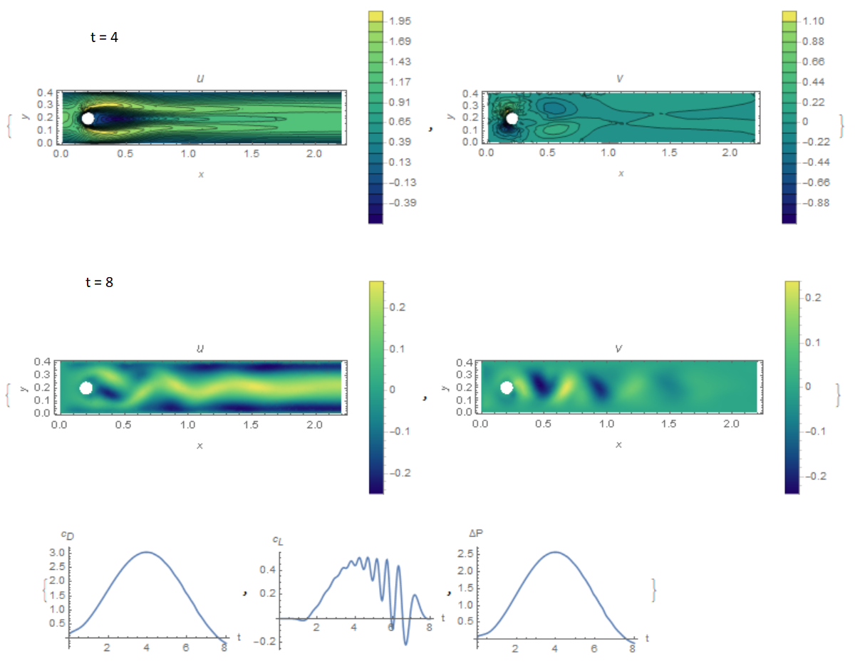
The next test differs from the previous one in that the input speed varies according to the U0[y_, t_] := 4*Um*y/H*(1 - y/H)*Sin[Pi*t/8]. It is necessary to determine the time dependence of the drag and lift parameters for a half-period of oscillation, as well as the pressure drop at the last moment of time. In Fig. 2 shows the components of the flow velocity and the required coefficients. Our solution of the problem and what is required in the test

sol = {3.0438934441256595`, 
   0.5073345082785012`, -0.11152933279750943`};

lowerbound = {2.9300, 0.4700, -0.1150};
upperbound = {2.9700, 0.4900, -0.1050};

Fig2 For this test, the agreement with the data in Table 5 is good. Consequently, the two tests are almost completely passed. I wrote and debugged this code using Mathematics 11.01. But when I ran this code using Mathematics 11.3, I got strange pictures, for example, the disk is represented as a hexagon, the size of the area is changed. Fig3 
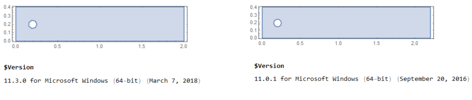
In addition, the numerical solution of the problem has changed, for example, test 2D2

{3.17805, 1.03297, 0.266606, 2.60427} v11.01
{3.15711, 1.11377, 0.266043, 2.54356} v11.03

The attached file contains the working code for test 2D3 describing the flow around the cylinder in a flat channel with a change in the flow velocity.

35 Replies

The latest versions of Mathematica allows as to calculate convection even with $Ra=10^7$. Data below has been computed with the code in the attached file. It takes a time to finish computation at t=1. Code has been developed by Lion Sahara and debugged here in my answer. In the picture below shown velocity field animated with step dt=0.01. We see the turbulent like convection
Figure 1.

Discussion and full code here:
Convection of air with higher Rayleigh number
https://community.wolfram.com/groups/-/m/t/3115061

Posted 1 month ago

Thank you very much. This is very helpful.

POSTED BY: Lion Sahara

Hi Alexander, Two quick questions:

1) Would it be possible to replace the cylinder by a square rod and still get a meaningful result? Or does this raise the turbulence to a level that either drives the CPU time to crazy values, or else becomes unstable?

2) Can Mathematica 12.1 also solve the unsteady compressible flow problem with temperatures in 3D (the problem with the cold cylinder and then computing several time steps, as you demonstrated further above)?

Cheers, Ron

Hi, Sorry, I already found it myself in the Wolfram online list of new features in Version 12:

3D Transient Fluid Flow and Energy Transport

Amazing! Cheers, Ron

Anonymous User
Anonymous User
Posted 4 years ago

Under the DFG Priority Research Program “Flow Simulation on High Performance Com- puters” solution methods for various flow problems have been developed

Someone above said "interesting to use old book equations and have mathematica show it" ... the above paper cited is not "old". Infact it does mostly to notate the speed of methods not show how it is solved (meaning, how to solve it).

My request is this. This is a great post for anyone to see. But "for the rest of us" it should be said at the beginning of the post if this is a heat conservation equations (or set of) or fluid flow conservation, if solved by fem instead system of pde matrix (if a choice), if this is heat flowing around a circular obstruction (what is the round thing, has it a temperature or it is a fluid obstruction) ... you know.

In other words for us beginners, please explain in english what we are physically representing / seeing and discuss if FEM is the only Mathematica solution, or if, say, monte carlo might be be easier and still show a plot (what do we get by using fem?). Explain setting up problem maybe (well, maybe a little complicated for that).

The cited .pdf file uses language which not everyone is going to know, like "laminar flow". on 2nd reading I see just above equations "fluid" is mentioned in just one sentence, easy to miss.

POSTED BY: Anonymous User

These are routine tests that I did for Mathematica FEM in version 11 using a special time integration algorithm that I am testing. Surprisingly, the tests were passed both in the problem of covection and in the problem of flow around a cylinder (these tests are quite complex and not every method can be used). I demonstrated other applications of the method on https://mathematica.stackexchange.com/

"12.0.0 for Mac OS X x86 (64-bit) (April 7, 2019)"

POSTED BY: Gobithaasan R.U.

OK! I will try to create a more robust algorithm. In this version, you can try t0=1/100.

Hi Alexander, Yes, the streamflow looks like a mess in V12 as attached. Any idea why such a case and how would i be able to get the right flow?

Thank, appreciate it. GR

Attachments:

I have this test running successfully on version 12. What is your version? Use $Version.

Dear Alexander,

I couldn’t have done it without you.

Thanks for being such a star :-)

POSTED BY: M.A. Ghorbani

I debugged the code. The file is attached. In version 12, the solution diverges on the right border, although in version 11 the solution converges.

Attachments:

Great. Thank you so much, Alexander :-)

May I have the used command or notebook for my future study?

I really appreciate your help.

POSTED BY: M.A. Ghorbani

Use this file with Mathematica 11.3. If you have questions ask here.

Attachments:
POSTED BY: M.A. Ghorbani

In fig. shows the laminar flow velocity profiles on a flat plate at $Re=800$. fig1

Mathematica FEM method can be used to calculate unsteady viscous compressible flows around aerofoil in subsonic, transonic and supersonic modes. Here an example is given for the wing profile NACA2415 for the Mach number $M = 0.55$, Reynolds number $Re = 1000$, angle of attack $\alpha =\pi/16$ .

myNACA[{m_, p_, t_}, x_] := 
  Module[{}, 
   yc = Piecewise[{{m/p^2 (2 p x - x^2), 
       0 <= x < p}, {m/(1 - p)^2 ((1 - 2 p) + 2 p x - x^2), 
       p <= x <= 1}}];
   yt = 5 t (0.2969 Sqrt[x] - 0.1260 x - 0.3516 x^2 + 0.2843 x^3 - 
       0.1015 x^4);
   \[Theta] = 
    ArcTan@Piecewise[{{(m*(2*p - 2*x))/p^2, 
        0 <= x < p}, {(m*(2*p - 2*x))/(1 - p)^2, p <= x <= 1}}];
   {{x - yt Sin[\[Theta]], 
     yc + yt Cos[\[Theta]]}, {x + yt Sin[\[Theta]], 
     yc - yt Cos[\[Theta]]}}];

m = 0.04;
p = 0.4;
tk = 0.15;
pe = myNACA[{m, p, tk}, x];
ParametricPlot[pe, {x, 0, 1}, ImageSize -> Large, Exclusions -> None]

ClearAll[myLoop];
myLoop[n1_, n2_] := 
 Join[Table[{n, n + 1}, {n, n1, n2 - 1, 1}], {{n2, n1}}]
Needs["NDSolve`FEM`"];
rt = RotationTransform[-\[Pi]/16];(*angle of attack*)a = 
 Table[pe, {x, 0, 1, 
   0.01}];
p0 = {p, 
      tk/2};
x1 = -2; x2 = 3;
y1 = -2; y2 = 2;
coords = 
     Join[{{x1, y1}, {x2, y1}, {x2, y2}, {x1, y2}}, rt@a[[All, 2]], 
      rt@Reverse[a[[All, 1]]]];
    nn = Length@coords;
    bmesh = ToBoundaryMesh["Coordinates" -> coords, 
       "BoundaryElements" -> {LineElement[myLoop[1, 4]], 
         LineElement[myLoop[5, nn]]}, "RegionHoles" -> {rt@p0}];
    mesh = ToElementMesh[bmesh, MaxCellMeasure -> 0.001];
Show[mesh["Wireframe"], Frame -> True]

q = 1.4;
k = 40; Re0 = 1; U0 = 1; M0 = 0.55; Re1 = Re0/M0^2; Pin = 1;
t0 = 1/20; alpha = 0;
UX[0][x_, y_] := Cos[alpha];
VY[0][x_, y_] := Sin[alpha];
\[CapitalRho][0][x_, y_] := Pin;
yU = Interpolation[rt@a[[All, 1]], InterpolationOrder -> 2];
yL = Interpolation[rt@a[[All, 2]], InterpolationOrder -> 2];
Do[
  {UX[i], VY[i], \[CapitalRho][i]} = 
   NDSolveValue[{{Inactive[
           Div][({{-\[Mu], 0}, {0, -\[Mu]}}.Inactive[Grad][
             u[x, y], {x, y}]), {x, y}] + 
         Re1*(Abs[\[CapitalRho][i - 1][x, y]]^q)*
\!\(\*SuperscriptBox[\(\[Rho]\), 
TagBox[
RowBox[{"(", 
RowBox[{"1", ",", "0"}], ")"}],
Derivative],
MultilineFunction->None]\)[x, y]/\[CapitalRho][i - 1][x, y] + 
         Re0*UX[i - 1][x, y]*D[u[x, y], x] + 
         Re0*VY[i - 1][x, y]*D[u[x, y], y] + 
         Re0*(u[x, y] - UX[i - 1][x, y])/t0, 
        Inactive[
           Div][({{-\[Mu], 0}, {0, -\[Mu]}}.Inactive[Grad][
             v[x, y], {x, y}]), {x, y}] + 
         Re1*(Abs[\[CapitalRho][i - 1][x, y]^q])*
\!\(\*SuperscriptBox[\(\[Rho]\), 
TagBox[
RowBox[{"(", 
RowBox[{"0", ",", "1"}], ")"}],
Derivative],
MultilineFunction->None]\)[x, y]/\[CapitalRho][i - 1][x, y] + 
         Re0*UX[i - 1][x, y]*D[v[x, y], x] + 
         Re0*VY[i - 1][x, y]*D[v[x, y], y] + 
         Re0*(v[x, y] - VY[i - 1][x, y])/t0, 
        D[\[CapitalRho][i - 1][x, y]*u[x, y], x] + 
         D[\[CapitalRho][i - 1][x, y]*v[x, y], 
          y] + (\[Rho][x, y] - \[CapitalRho][i - 1][x, y])/t0} == {0, 
        0, 0} /. \[Mu] -> 1/1000, {
      DirichletCondition[{u[x, y] == U0*Cos[alpha], 
        v[x, y] == U0*Sin[alpha]}, x == x1 && y1 < y < y2], 
      DirichletCondition[{u[x, y] == 0., v[x, y] == 0.}, 
       y == yU[x] && 0 <= x <= Cos[Pi/16]], 
      DirichletCondition[{u[x, y] == 0., v[x, y] == 0.}, 
       y == yL[x] && 0 <= x <= Cos[Pi/16]],
      DirichletCondition[\[Rho][x, y] == 1, x == x2]}}, {u, 
     v, \[Rho]}, {x, y} \[Element] mesh, 
    Method -> {"FiniteElement", 
      "InterpolationOrder" -> {u -> 2, v -> 2, \[Rho] -> 1}}], {i, 1, 
   k}];

ContourPlot[
Norm[{UX[i][x, y], VY[i][x, y]}] /. i -> 32, {x, x1, x2}, {y, y1, 
y2}, PlotLegends -> Automatic, Contours -> 20, 
ColorFunction -> "TemperatureMap", FrameLabel -> {"x", "y"}, 
PlotLabel -> V, PlotRange -> All, PlotPoints -> 50, MaxRecursion -> 2]

sp = StreamPlot[{UX[i][x, y], VY[i][x, y]} /. i -> 32, {x, -0.5, 
1.5}, {y, -.5, .5}, PlotLegends -> Automatic, 
ColorFunction -> "TemperatureMap", FrameLabel -> {"x", "y"}, 
PlotLabel -> V, PlotRange -> All, MaxRecursion -> 2, 
StreamStyle -> LightGray, StreamPoints -> Fine, 
AspectRatio -> Automatic];
cp = ContourPlot[
Norm[{UX[i][x, y], VY[i][x, y]}] /. i -> 32, {x, -0.5, 
1.5}, {y, -.5, .5}, PlotLegends -> Automatic, 
ColorFunction -> "BlueGreenYellow", FrameLabel -> {"x", "y"}, 
PlotLabel -> V, PlotRange -> All, MaxRecursion -> 2, 
Contours -> 40, AspectRatio -> Automatic, PlotPoints -> 50];

Show[cp, sp]
StreamPlot[{UX[i][x, y], VY[i][x, y]} /. i -> 32, {x, 0.9, 
  1.05}, {y, -0.22, -0.12}, Epilog -> {Line[coords[[5 ;; nn]]]}, 
 AspectRatio -> Automatic, StreamPoints -> Fine]

fig1

Hi Alexander, I get the following error while trying to run the code using version 12. How can i fix it?

##### NDSolveValue::overdet: There are fewer dependent variables, {[Rho][x,y]}, than equations, so the system is overdetermined. Set::shape: Lists {UX[i],VY[i],[CapitalRho][i]} and NDSolveValue[<<1>>] are not the same shape.

######## Thanks! gr

Attachments:

Very nice example, thank you Alexander. I'd like to combine some features of the two models and simulate forced convection in air onto a cylinder in 2D (as in the above examples in this post), but with a temperature difference between cylinder and air. Optimally, there should be no walls (or the simulation domain should be quite large, if "no walls" boundary conditions are unstable). I'm interested in the air temperature distribution in the wake, i.e., after the air has exchanged heat with the cylinder, given a certain convective surface conduction value (unit W/m^2/K) on the cylinder wall. The Reynolds number should be rather high, but below 5 x 10^5, i.e., before the onset of full turbulence. Cheers, Ron

Posted 5 years ago

There are two different models - an incompressible viscous flow at $Re=100$ and convection in the Boussinesq approximation in a rectangular cavity with a Rayleigh number of $Ra=10^3, 10^4,10^5$. Transition to turbulence in the wake of the cylinder in 3D occurs already at $Re=170-260$. We can put $Re = 1000$ so that everything is mixed in the wake. In what approximation do you want to calculate convection? How is the cylinder oriented relative to the vertical?

POSTED BY: Updating Name

I consulted a textbook on boundary layer flow which states that the turbulence onset on the surface is at Re = 5 x 10^5. It may well be that turbulence in the wake starts earlier.

The cylinder axis is vertical to the convection direction, as in your first example. The cylinder has a diameter of, say, 60 cm, and is a few Kelvin cooler than the incoming air. I'd like to model the resulting air cooling pattern in space and time.

I'm not sure which approximation to choose, I'm not an expert on CFD -- that's why I'm asking in this forum.

In fig. shows the temperature at various points in time when hot air flows around a cold cylinder at $Re=10^3$. fig1

Thanks for the 2D flow simulation around the cooled cylinder, Alexander.

Would you be able to send me the Mathematica code that you used?

Thanks, Ron

In the attached file, the code for version 11.01 is using linear FEM . I can rewrite the code for version 12 using non-linear FEM to reduce the time.

Attachments:

Using the nonlinear solver would be great indeed, Alexander! Cheers, Ron

I tested this method of solution on the problems of natural convection. Here we give three tests for the problem of natural convection of air in a rectangular cavity with a Rayleigh number of $Ra=10^3,10^4, 10^5$. On the side walls of the cavity a constant temperature difference is maintained, the upper and lower walls are thermally insulated. We use the Boussinesq approximation. As a standard, we use the data from the article:

Vahl Davis, G.de (1983) : Natural convection of air in a square cavity : A bench mark numerical solution. Int. J. Numer. Methods Fluids 3, 249-264.

Coincidence in all three tests is generally good. Thus, we showed the application of the method for solving the problems of thermal convection in the case of laminar flows. A system of equations describing free convection

$\nabla .\vec u=0, \frac{d\vec u}{dt}=Pr\nabla ^2\vec u -RaPrT\frac {\vec g}{g}$

$\frac {dT}{dt}=\nabla^2T$

$ d/dt =\partial/\partial t +(\vec u .\nabla )$

$\vec u$ is velocity field vector, $T$ - temperature, $\vec g $ - gravity vector, $Pr$ - the Prandtl number, $Ra$ - the Rayleigh number.

Code for the case $Pr=0.71, Ra=10^3$:

K = 100; Pr0 = .71; Ra = 10^3; R = Ra*Pr0; t0 = 1/100; a = 0;
\[CapitalOmega] = ImplicitRegion[0 <= x <= 1 && 0 <= y <= 1, {x, y}];;
UX[0][x_, y_] := 0;
VY[0][x_, y_] := 0;
\[CapitalRho][0][x_, y_] := 0;
TK[0][x_, y_] := 0; TX[0][x_, y_] := 0;
Do[
  {UX[i], VY[i], \[CapitalRho][i], TK[i], TX[i]} = 
   NDSolveValue[{{Inactive[
           Div][({{-\[Mu], 0}, {0, -\[Mu]}}.Inactive[Grad][
             u[x, y], {x, y}]), {x, y}] + D[p[x, y], x] + 
         UX[i - 1][x, y]*D[u[x, y], x] + 
         VY[i - 1][x, y]*D[u[x, y], y] + (u[x, y] - UX[i - 1][x, y])/
          t0 - R*T[x, y]*Sin[a], 
        Inactive[
           Div][({{-\[Mu], 0}, {0, -\[Mu]}}.Inactive[Grad][
             v[x, y], {x, y}]), {x, y}] + D[p[x, y], y] + 
         UX[i - 1][x, y]*D[v[x, y], x] + 
         VY[i - 1][x, y]*D[v[x, y], y] - 
         R*T[x, y]*Cos[a] + (v[x, y] - VY[i - 1][x, y])/t0, 
        D[u[x, y], x] + D[v[x, y], y]} == {0, 0, 0} /. \[Mu] -> Pr0, {
      DirichletCondition[{p[x, y] == 0}, y == 1 && x == 1], 
      DirichletCondition[{u[x, y] == 0, v[x, y] == 0}, 
       y == 0 || y == 1]}, {UX[i - 1][x, y]*D[T[x, y], x] + 
        VY[i - 1][x, y]*D[T[x, y], y] + (T[x, y] - TK[i - 1][x, y])/
         t0 - (D[T[x, y], x, x] + D[T[x, y], y, y]) == 
       NeumannValue[0, y == 0 || y == 1], 
      DirichletCondition[{u[x, y] == 0, v[x, y] == 0, T[x, y] == 1}, 
       x == 0], 
      DirichletCondition[{u[x, y] == 0, v[x, y] == 0, T[x, y] == 0}, 
       x == 1]}}, {u, v, p, T, 
\!\(\*SuperscriptBox[\(T\), 
TagBox[
RowBox[{"(", 
RowBox[{"1", ",", "0"}], ")"}],
Derivative],
MultilineFunction->None]\)}, {x, y} \[Element] \[CapitalOmega], 
    Method -> {"FiniteElement", 
      "InterpolationOrder" -> {u -> 2, v -> 2, p -> 1, T -> 2}, 
      "MeshOptions" -> {"MaxCellMeasure" -> 0.001}}], {i, 1, K}];
{ContourPlot[TK[K][x, y], {x, y} \[Element] \[CapitalOmega], 
PlotLegends -> Automatic, Contours -> 20, PlotPoints -> 25, 
ColorFunction -> "TemperatureMap", AxesLabel -> {"x", "y"}, 
PlotLabel -> T], 
StreamDensityPlot[{UX[K][x, y], 
VY[K][x, y]}, {x, y} \[Element] \[CapitalOmega], 
StreamPoints -> Fine, StreamStyle -> LightGray, 
PlotLegends -> Automatic, VectorPoints -> Fine, 
ColorFunction -> "TemperatureMap", PlotLabel -> Row[{"Ra=", Ra}]]}

MaximalBy[Table[{x, VY[K][x, .5]}, {x, 0, 1, .0001}], Last]

 {{0.1787, 3.69762}}

(*BenchmarkCase={x=0.178,vmax=3.697}*)

 MaximalBy[Table[{y, UX[K][0.5, y]}, {y, 0, 1, .0001}], Last]

 {{0.8132, 3.64937}}

 (*BenchmarkCase={y=0.813,umax=3.649}*)


 MaximalBy[Table[{y, -TX[K][0, y]}, {y, 0, 1, 0.0001}], Last]

 {{0.0909, 1.50724}}

 (*BenchmarkCase={y=0.092,Numax=1.505}*)

 NuAv = 
 NIntegrate[
  UX[K][x, y]*TK[K][x, y] - TX[K][x, y], {x, 0, 1}, {y, 0, 1}, 
  WorkingPrecision -> 5]

 1.1159

 (*BenchmarkCase=1.118*)


 Nu0 =  NIntegrate[-TX[K][0, y], {y, 0, 1}, WorkingPrecision -> 5]

 1.1182

(*BenchmarkCase=1.117*)

 Nu05 = 
 NIntegrate[UX[K][.5, y]*TK[K][.5, y] - TX[K][0.5, y], {y, 0, 1}, 
  WorkingPrecision -> 5]

1.1179

 (*BenchmarkCase=1.118*)

MinimalBy[Table[{y, -TX[K][0, y]}, {y, 0, 1, 0.0001}], Last]

 {{1., 0.691182}}

 (*BenchmarkCase={y=1,Numin=0.692}*)

fig1

Thank you for the kind words, Alexander! It is always great to hear our user are excited about Wolfram Technologies. I am looking forward to more of your wonderful posts on Wolfram Community using this tech :-)

POSTED BY: Vitaliy Kaurov
Posted 5 years ago

Thank you, Vitaliy! I'm trying to pass two tests for the cylinder, which are described above, using nonlinear FEM. I will report the results here.

POSTED BY: Updating Name

Thanks for it! It is pretty amazing and fun to see that some, for example textbook-scope, fluid mechanics example simulations can be carried out in Mathematica, i.e. by way of pure coding and then hitting the Shift+Enter button.

Needless to comment that for fluid mechanics simulations in any slightly more complicated 2-D geometries or RL 3-D geometries, one would resort to a GUI-driven software where the user interacts with the mouse and context menus and does not have to code anything. Often enough I miss GUI interactivity (similar to Word, Excel. PowerPoint, Comsol) in our software, but then I also realize that Mathematica grants more flexibility and direct control over other details which can't be manipulated in those specialized user-friendly applications.

The bottom line is that for each task at hand one should choose the proper tool wisely. Me too, i enjoy trying to use the software for all and everything at least once. Good for my coding learning experience.

POSTED BY: Raspi Rascal

I express my gratitude to the Moderation Team for appreciating my work. I'll add an animation for the 2D2 test here and the Navier-Stokes for an unsteady flow with an explanation of the statement of the problem for tests 2D2 and 2D3 from the cited article of M. Schäfer and S. Turek

fig7

fig8

Would be helpful to see the mathematical equations and conditions in traditional textbook format. Also would be helpful to see the animation of the fluid from t=0…100s

POSTED BY: Raspi Rascal

enter image description here - Congratulations! This post is now a Staff Pick as distinguished by a badge on your profile! Thank you, keep it coming!

POSTED BY: Moderation Team

The Euler method is a poor way to solve a differential equation. It can be numerically unstable.

POSTED BY: Frank Kampas
Reply to this discussion
Community posts can be styled and formatted using the Markdown syntax.
Reply Preview
Attachments
Remove
or Discard

Group Abstract Group Abstract