Tuseeta-san's post is how to convert a trained model of TensorFlow to Mathematica. Converting trained models from a language other than Mathematica to Mathematica is very beneficial to Mathematica users. So I'll show how to convert a trained model of PyTorch to Mathematica along with Tuseeta-san's post.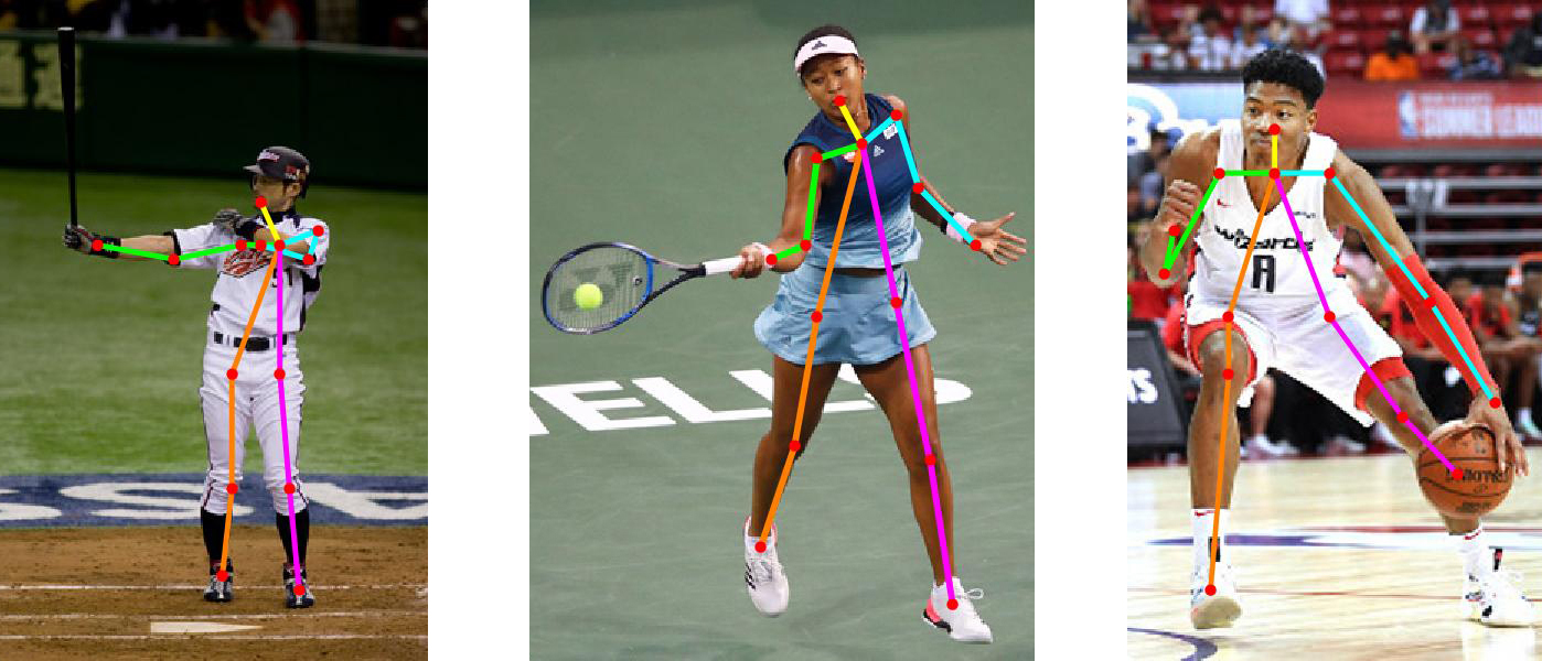

Step 1: Figure out the architecture

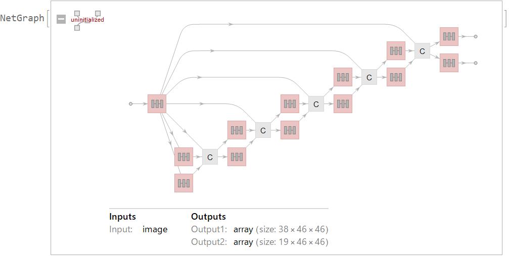
The model to be converted is Pose Estimation that detects the human skeleton (body parts and their connections) from an image. It's called OpenPose.The model consists of Feature map that extracts image features and six Stage maps. Feature map extracts image features from an input image(size:368*368). Each Stage map has two-branch, the first branch predicts confidence and the second predicts PAFs?Part Affinity Fields), along with the image feature .Two-branch are concatenated for next stage.

Step 2: Coding it in Mathematica

Feature map

The Feature map consists of the first 23 layers of VGG-19, followed by 2 sets of Convolution and Ramp.

Extract the first 23 layers of VGG-19.

vgg19 = NetModel["VGG-19 Trained on ImageNet Competition Data"];
vgg19sub = Take[vgg19, {1, 23}];

Change Encoder.

enc = NetExtract[vgg19, "Input"];
enc = NetReplacePart[
   enc, {"ImageSize" -> {368, 368}, 
    "VarianceImage" -> {0.229, 0.224, 0.225}, 
    "MeanImage" -> {0.485, 0.456, 0.406}}];
featurefirst = NetReplacePart[vgg19sub, "Input" -> enc];

Add Convolution and Ramp.

feature = 
  NetAppend[
   featurefirst, {"convadd1" -> 
     ConvolutionLayer[256, 3, "Stride" -> 1, "PaddingSize" -> 1], 
    "reluadd1" -> Ramp,
    "convadd2" -> 
     ConvolutionLayer[128, 3, "Stride" -> 1, "PaddingSize" -> 1], 
    "reluadd2" -> Ramp}];

Stage map

Each Stage map consists only of Convolutions and Ramps.

Stage 1: The differences between two branches is that the last output channel number is 38 or 19.

blk11 = NetChain[{
    ConvolutionLayer[128, 3, "Stride" -> 1, "PaddingSize" -> 1], Ramp,
    ConvolutionLayer[128, 3, "Stride" -> 1, "PaddingSize" -> 1], Ramp,
    ConvolutionLayer[128, 3, "Stride" -> 1, "PaddingSize" -> 1], Ramp,
    ConvolutionLayer[512, 1, "Stride" -> 1, "PaddingSize" -> 0], Ramp,
    ConvolutionLayer[38, 1, "Stride" -> 1, "PaddingSize" -> 0]}];
blk12 = NetChain[{
    ConvolutionLayer[128, 3, "Stride" -> 1, "PaddingSize" -> 1], Ramp,
    ConvolutionLayer[128, 3, "Stride" -> 1, "PaddingSize" -> 1], Ramp,
    ConvolutionLayer[128, 3, "Stride" -> 1, "PaddingSize" -> 1], Ramp,
    ConvolutionLayer[512, 1, "Stride" -> 1, "PaddingSize" -> 0], Ramp,
    ConvolutionLayer[19, 1, "Stride" -> 1, "PaddingSize" -> 0]}];

Stage 2?6: The difference between Stage1 and Stage2?6 is the kinds and the numbers of layers.

blkx1 = NetChain[{
    ConvolutionLayer[128, 7, "Stride" -> 1, "PaddingSize" -> 3], Ramp,
    ConvolutionLayer[128, 7, "Stride" -> 1, "PaddingSize" -> 3], Ramp,
    ConvolutionLayer[128, 7, "Stride" -> 1, "PaddingSize" -> 3], Ramp,
    ConvolutionLayer[128, 7, "Stride" -> 1, "PaddingSize" -> 3], Ramp,
    ConvolutionLayer[128, 7, "Stride" -> 1, "PaddingSize" -> 3], Ramp,
    ConvolutionLayer[128, 1, "Stride" -> 1, "PaddingSize" -> 0], Ramp,
    ConvolutionLayer[38, 1, "Stride" -> 1, "PaddingSize" -> 0]}];
blkx2 = NetChain[{
    ConvolutionLayer[128, 7, "Stride" -> 1, "PaddingSize" -> 3], Ramp,
    ConvolutionLayer[128, 7, "Stride" -> 1, "PaddingSize" -> 3], Ramp,
    ConvolutionLayer[128, 7, "Stride" -> 1, "PaddingSize" -> 3], Ramp,
    ConvolutionLayer[128, 7, "Stride" -> 1, "PaddingSize" -> 3], Ramp,
    ConvolutionLayer[128, 7, "Stride" -> 1, "PaddingSize" -> 3], Ramp,
    ConvolutionLayer[128, 1, "Stride" -> 1, "PaddingSize" -> 0], Ramp,
    ConvolutionLayer[19, 1, "Stride" -> 1, "PaddingSize" -> 0]}];

Finally, create OpenPose.

openpose = NetGraph[{
   "feature" -> feature,(*feature*)
   "blk11" -> blk11, "blk12" -> blk12,(*stage 1*)
   "blk21" -> blkx1, "blk22" -> blkx2,(*stage 2*)
   "cat12" -> CatenateLayer[],
   "blk31" -> blkx1, "blk32" -> blkx2,(*stage 3*)
   "cat23" -> CatenateLayer[],
   "blk41" -> blkx1, "blk42" -> blkx2,(*stage 4*)
   "cat34" -> CatenateLayer[],
   "blk51" -> blkx1, "blk52" -> blkx2,(*stage 5*)
   "cat45" -> CatenateLayer[],
   "blk61" -> blkx1, "blk62" -> blkx2,(*stage 6*)
   "cat56" -> CatenateLayer[]
   },
  {"feature" -> "blk11", "feature" -> "blk12",(*stage 1*)
   {"blk11", "blk12", "feature"} -> "cat12",(*stage 2*)
   "cat12" -> "blk21", "cat12" -> "blk22",
   {"blk21", "blk22", "feature"} -> "cat23",(*stage 3*)
   "cat23" -> "blk31", "cat23" -> "blk32",
   {"blk31", "blk32", "feature"} -> "cat34",(*stage 4*)
   "cat34" -> "blk41", "cat34" -> "blk42",
   {"blk41", "blk42", "feature"} -> "cat45",(*stage 5*)
   "cat45" -> "blk51", "cat45" -> "blk52",
   {"blk51", "blk52", "feature"} -> "cat56",(*stage 6*)
   "cat56" -> "blk61", "cat56" -> "blk62"
   }]

Step 3: Importing the Weights and the Biases

Download "posemodelscratch.pth" as a trained model of PyTorch.

Import the parameters, the weights and the biases. I referred "How to import python pickle *.pkl?"

session = StartExternalSession["Python-NumPy"];
parameters = ExternalEvaluate[session, "import torch
import numpy as np
import pickle as pkl

net_weights = torch.load(
       'pose_model_scratch.pth', map_location={'cuda:0': 'cpu'})
keys = list(net_weights.keys())

parameters = {}
for i in range(len(keys)):
       t = net_weights[keys[i]]       
       x = t.numpy()
       parameters[keys[i]] = x.flatten()
parameters"];
DeleteObject[session];

keys = Keys[parameters];
parameters = Values[parameters];

Step 4: Parsing the Weights and the Biases

The parameters is 184 sets of one-dimensional lists. They consists of the Weights and the Biases of 92 Convolution layers in OpenPose.

Get a list of layer names for OpenPose with depth level. Then, get a list of 92 names where convolution layer is used in it.

layernames = 
  GroupBy[Keys@NetInformation[openpose, "Layers"], First] // Values;
convlayernames = (Position[
     NetInformation[openpose, "Layers"], _ConvolutionLayer] // 
    Flatten)[[All, 1]]

As you can see in keys, you can see that the order of convolution layers of OpenPose is different from the order of convolution layers of "posemodelscratch.pth"

 keys

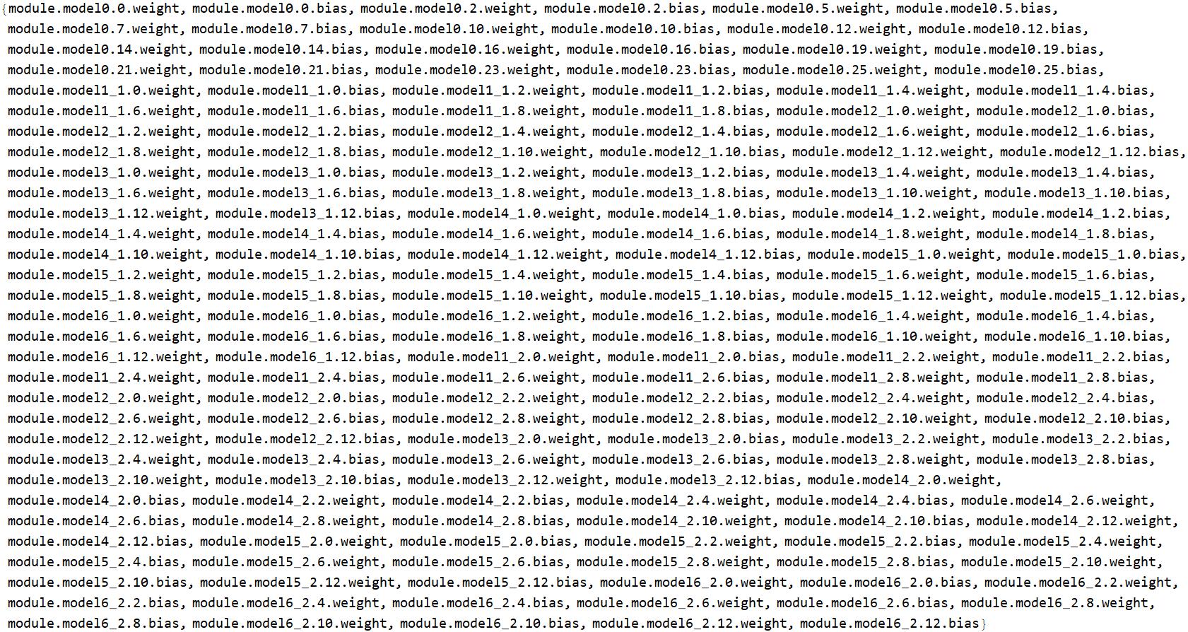
So, manually sort the order of convolution layers in OpenPose into the order of "posemodelscratch.pth"

convlayernamesGH = {{"feature", "conv1_1"}, {"feature", "conv1_2"},
   {"feature", "conv2_1"}, {"feature", "conv2_2"},
   {"feature", "conv3_1"}, {"feature", "conv3_2"}, {"feature", "conv3_3"}, {"feature", "conv3_4"},
   {"feature", "conv4_1"}, {"feature", "conv4_2"},
   {"feature", "convadd1"}, {"feature", "convadd2"},
   {"blk11", 1}, {"blk11", 3}, {"blk11", 5}, {"blk11", 7}, {"blk11", 9},
   {"blk21", 1}, {"blk21", 3}, {"blk21", 5}, {"blk21", 7}, {"blk21", 9}, {"blk21", 11}, {"blk21", 13},
   {"blk31", 1}, {"blk31", 3}, {"blk31", 5}, {"blk31", 7}, {"blk31", 9}, {"blk31", 11}, {"blk31", 13},
   {"blk41", 1}, {"blk41", 3}, {"blk41", 5}, {"blk41", 7}, {"blk41", 9}, {"blk41", 11}, {"blk41", 13},
   {"blk51", 1}, {"blk51", 3}, {"blk51", 5}, {"blk51", 7}, {"blk51", 9}, {"blk51", 11}, {"blk51", 13},
   {"blk61", 1}, {"blk61", 3}, {"blk61", 5}, {"blk61", 7}, {"blk61", 9}, {"blk61", 11}, {"blk61", 13},
   {"blk12", 1}, {"blk12", 3}, {"blk12", 5}, {"blk12", 7}, {"blk12", 9},
   {"blk22", 1}, {"blk22", 3}, {"blk22", 5}, {"blk22", 7}, {"blk22", 9}, {"blk22", 11}, {"blk22", 13},
   {"blk32", 1}, {"blk32", 3}, {"blk32", 5}, {"blk32", 7}, {"blk32", 9}, {"blk32", 11}, {"blk32", 13},
   {"blk42", 1}, {"blk42", 3}, {"blk42", 5}, {"blk42", 7}, {"blk42", 9}, {"blk42", 11}, {"blk42", 13},
   {"blk52", 1}, {"blk52", 3}, {"blk52", 5}, {"blk52", 7}, {"blk52", 9}, {"blk52", 11}, {"blk52", 13},
   {"blk62", 1}, {"blk62", 3}, {"blk62", 5}, {"blk62", 7}, {"blk62", 9}, {"blk62", 11}, {"blk62", 13}
   };

Get the position of each element of convlayernamesGH in OpenPose.

convlayerpos = 
 Flatten[Position[layernames, #] & /@ convlayernamesGH, 1]

Reshape each one-dimensional list of parameters to the dimension of the corresponding weight or bias.

getDimB[layer_] := Dimensions@NetExtract[layer, "Biases"]
getDimW[layer_] := Dimensions@NetExtract[layer, "Weights"]
convs = NetExtract[NetInitialize[openpose], #] & /@ convlayerpos;
dimW = getDimW /@ convs;
dimB = getDimB /@ convs;
dim = Flatten[Transpose[{dimW, dimB}], 1];
parametersReshape = MapThread[ArrayReshape, {parameters, dim}];

Step 5: Linking the Weights and the Biases

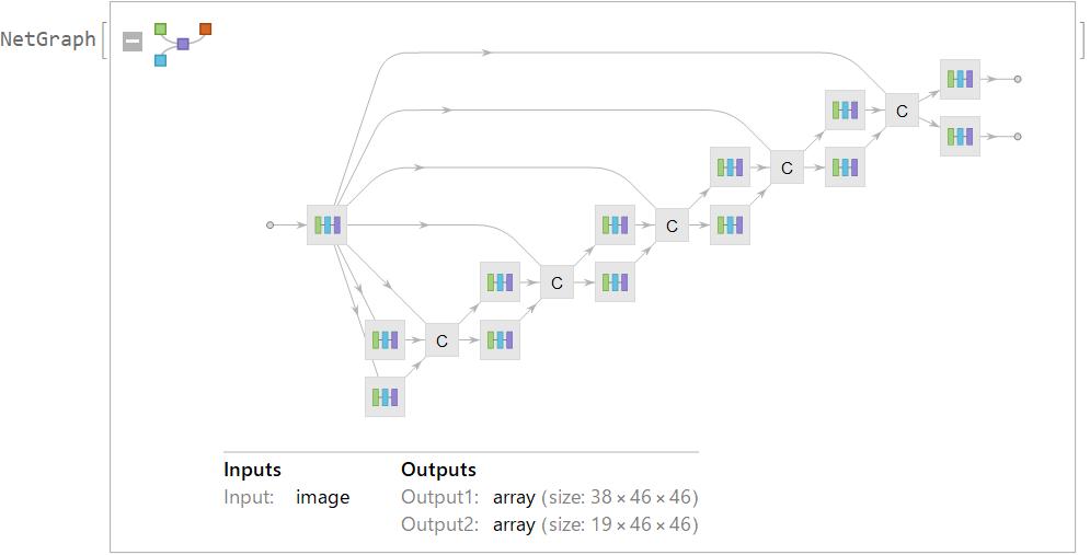
Replace the initial values of weights and biases in OpenPose with learned parameters, and finally get trained OpenPose.

replacenames =
  Flatten[
   Transpose[{Flatten@{#, "Weights"} & /@ convlayernamesGH, 
     Flatten@{#, "Biases"} & /@ convlayernamesGH}], 1];
rule = Thread[replacenames -> parametersReshape];
trainedOpenPose = NetReplacePart[openpose, rule]

Step 6: Making the tests

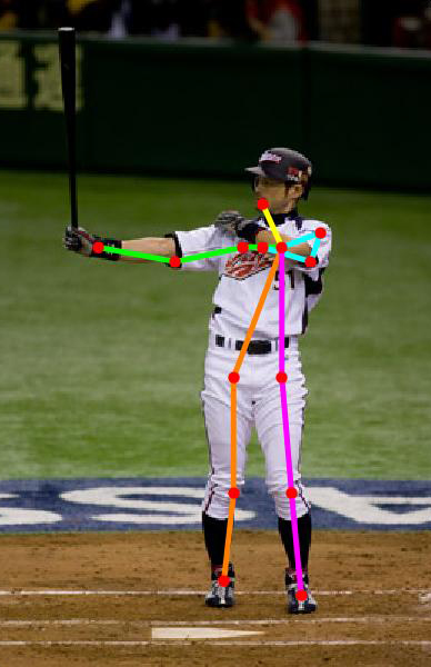
For simplification, estimate pose for the image of single-person. The Output2 of OpenPose shows the confidence of 19 body parts in each part where the image is divided into 46 * 46.

1:Nose, 2:Neck, 3:RShoulder, 4:RElbow, 5:RWrist, 6:LShoulder, 7:LElbow, 8:LWrist, 9:RHip, 10:RKnee, 11:RAnkle, 12:LHip, 13:LKnee, 14:LAnkle, 15:REye, 16:LEye, 17:REar, 18:LEar, 19:Bkg

Define the function to get the position of max of confidence of each body part.

maxpts[img_, confidences_, idex_] := Module[{pos, pts, h},
  pos = Reverse@First@Position[h = confidences[[idex]], Max@h];
  pts = (pos/46)*ImageDimensions@img; 
  pts = {pts[[1]], (ImageDimensions@img)[[2]] - pts[[2]]}
  ]

Connect the detected body parts and show the result together on the original image.

showpose[img_] := Module[{bodylist, size, out, confidences, pts, pose},
  bodylist = {1, 2, 3, 4, 5, 6, 7, 8, 9, 10, 11, 12, 13, 14};
  size = {368, 368};
  out = trainedOpenPose[img];
  confidences = out[[2]];
  pts = maxpts[img, confidences, #] & /@ bodylist;
  pose = Graphics[{
     Yellow, Thickness[.0125], Line[pts[[#]] & /@ {1, 2}],
     Green, Line[pts[[#]] & /@ {2, 3, 4, 5}],
     Cyan, Line[pts[[#]] & /@ {2, 6, 7, 8}],
     Orange, Line[pts[[#]] & /@ {2, 9, 10, 11}],
     Magenta, Line[pts[[#]] & /@ {2, 12, 13, 14}],
     PointSize[Large], Red, Point[pts],
     White, Point[{{0, 0}, ImageDimensions@img}]
     }, ImagePadding -> All];
  Show[img, pose]
  ]

Let' try.

img = Import["ichiro.jpg"];
showpose[img]

Future work

? Estimate the pose of an image in which multi-person are by using PAFs of output1 of OpenPose.

? Convert a more accurate pose estimation model.

Attachments:

openpose.nb