Hi Neil,

Could you please point me to where you've seen the comment that ScalingFunction does not apply to any options? The only relevant comment that I've found in the documentation is one stating "Options are specified in the original coordinates". Which I've read as meaning that graphics coordinates specified in Prolog/Epilog and other option expressions should not need to be individually scaled. But, for the Epilog and Prolog options at least, the coordinates of graphics expressions do need to be scaled. From what you say, I may be missing something in the documentation. Or I could be completely misunderstanding it. Which is perfectly possible ;-)

Irrespective of what the documentation says, I think that when ScalingFunctions are specified they should be applied to the data and all options. I can't think of a case where this wouldn't be the intention and not doing so just presents us with a headache and unnecessary extra work.

For me, there seems to be some inconsistency in how ScalingFunctions are applied to options. This is illustrated in the attached notebook, which gives examples that show ScalingFunctions are not applied to the Prolog and Epilog options but are applied to the PlotRange option.

So, if this behaviour is not a bug and is intentional, as you suggest, my view is that it should be changed.

All the best,

Ian

Attachments:

ScalingFunctions.nb

Bug or not, who knows. For my point of view, it's not logical and pretty useless how it works now:

• Applied to Plot, but not Graphics.
• Not applied to Pro/Epilog, see Ian.

I don't know, how to reach Arnoud Buzing. I tried to place the issue at enter link description here

I think as well, that's a bug. I can't imagine any reason why not all coordinates could be transformed automatically by the ScalingFunctions-option. Nor that it is not supported in Graphics (but - surprise! - accepted). The underlying transformations are trivial.

Do you know, when 12.1 will arrive?

Thanks a lot, Henrik. This does what I want to do. I've stupidly overlooked the option ScalingFunctions so far.

Unfortunately, it works for the Plot-functions only, but not for Graphics. Strange enough, for Graphics it is accepted, marked red but ignored.

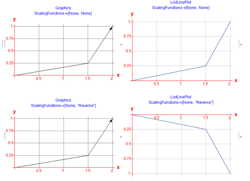
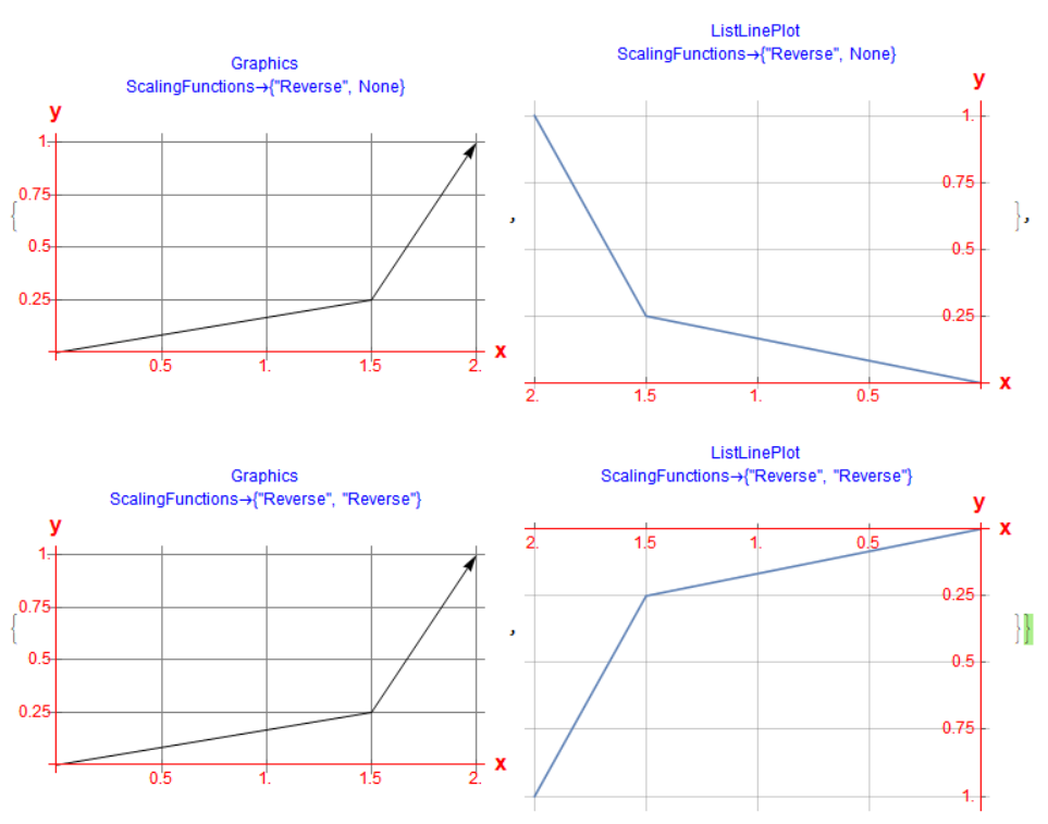
The following code draws a broken line with all four axis orientations. Once with Graphics as an Arrow and once with ListLinePlot as a Line. Everything else is identical.

You can see that ListLinePlot does everything right. (Maybe except for the AxesLabel, which are not placed at the correct position at the end of the axis).

Block[{graphs, i, pts, xticks, yticks},
 pts = {{0, 0}, {1.5, 0.25}, {2, 1}};
 xticks = 0.5*Range[4]; yticks = 0.25*Range[4];
 graphs = Table[{Null, Null}, 4]; i = 0;
 Do[i++;
  graphs[[i, 1]] = Graphics[Arrow[pts]
    , Axes -> True, AxesStyle -> Directive[Red, 12], 
    ScalingFunctions -> sfs
    , AxesLabel -> (Style[#, Red, Bold, 16] & /@ {"x", "y"})
    , Ticks -> {xticks, yticks}, GridLines -> {xticks, yticks}
    , PlotLabel -> 
     Style[Column[{"Graphics", 
        Row[{"ScalingFunctions\[Rule]", sfs // InputForm}]}, Center], 
      Blue]
    , ImageSize -> Medium];
  graphs[[i, 2]] = ListLinePlot[pts
    , Axes -> True, AxesStyle -> Directive[Red, 12], 
    ScalingFunctions -> sfs
    , AxesLabel -> (Style[#, Red, Bold, 16] & /@ {"x", "y"})
    , Ticks -> {xticks, yticks}, GridLines -> {xticks, yticks}
    , PlotLabel -> 
     Style[Column[{"ListLinePlot", 
        Row[{"ScalingFunctions\[Rule]", sfs // InputForm}]}, Center], 
      Blue]
    , ImageSize -> Medium]
  , {sfs, {{None, None}, {None, "Reverse"}, {"Reverse", 
     None}, {"Reverse", "Reverse"}}}
  ];
 Print[graphs]
 ]

Hi Werner,

You could try the undocumented Charting`ScaledTicks function.

Graphics[Circle[{2, -2}, 1], Axes -> True, AxesOrigin -> {0, 0}, 
 Ticks -> {Automatic, Charting`ScaledTicks["Reverse"][##, {12, 6}] &}]

But note that you will have to flip the sign of all y coordinates {2, -2} above.

No. This are standard axes. y is running from the bottom (-3) to top (0).

What I want is y=0 on top and y=3 on the bottom. I.e. the standard way how by example screen display points are addressed (origin at top left).