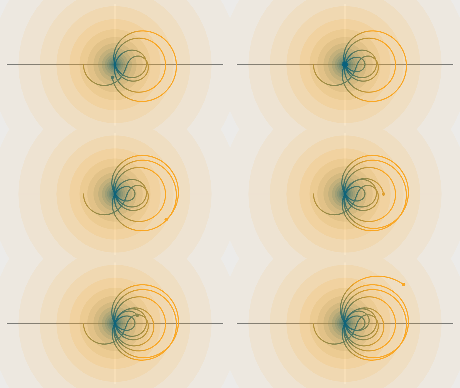
I just wanted to share Quanta Magazine's new explainer video on the Riemann Hypothesis, to which I contributed a number of animations: https://youtu.be/zlm1aajH6gY The full Quanta Magazine article can be found here: How I Learned to Love and Fear the Riemann Hypothesis.
Here's a GIF of part of the spiral animation :

And here's a Manipulate version of the spiral animation:
zetazeros = Table[N[Im[ZetaZero[i]]], {i, 1, 20}];

DynamicModule[{diffs, pos, xaxesLength = 5, yaxesLength = 9/16*5,
  range = 3, tmax = 55, axesColor,
  cols = RGBColor /@ {"#07617d", "#f9a828", "#2e383f", "#ececeb"},
  n = Length[zetazeros]},
 axesColor = cols[[3]];
 Manipulate[
  diffs = Table[a - zetazeros[[i]], {i, 1, n}];
  pos = Position[diffs, x_ /; 0 < x < 1];
  Show[Graphics[{axesColor, Thickness[.002],
     Line[{{-xaxesLength, 0}, {xaxesLength, 0}}],
     Line[{{0, -yaxesLength}, {0, yaxesLength}}],
     Reverse@Table[{Opacity[(8 - E^r)/48], Blend[cols[[;; 2]], E^r/2],
         Disk[{0, 0}, E^r]}, {r, -5, 5, 1/4}]}],
   ParametricPlot[ReIm[Zeta[1/2 + I t]], {t, 0, a},
    PlotStyle -> Directive[Thickness[.005], CapForm["Round"]],
    ColorFunctionScaling -> False,
    ColorFunction ->
     Function[{x, y, t}, Blend[cols[[;; 2]], Norm[{x, y}]/2]]],
   Graphics[{Blend[cols[[;; 2]], Abs[Zeta[1/2 + I a]]/2],
     PointSize[.015], Point[ReIm[Zeta[1/2 + I a]]], cols[[1]],
     If[Length[pos] >= 1, {Opacity[1 - diffs[[pos[[1, 1]]]]],
       Disk[{0, 0}, 2 diffs[[pos[[1, 1]]]]]}]}],
   ImageSize -> 50 {16, 9}, Background -> cols[[-1]],
   PlotRange -> range {{-16/9, 16/9}, {-1, 1}}],
  {a, .0001, tmax, (tmax - .0001)/840}]
 ]