
Recently we have worked a few examples showing that it's not too difficult to derive Cellular Automaton growth rules for substitution tilings of the plane. As discussed in the context of the Penrose tiling, computing atlases and their unique partial completions can expedite the process of deriving growth rules. The purpose of this memo is to work another example related to the Blue Tiling, a work of computer fractal art from a few years ago. Partial completions of the Blue Tiling obtained through the substitution rule already have a boundary reminiscent of snowflakes. At the end we can compare the new growth rule with the half-hex growth, and speculate briefly about agreement with microscopic data.
We will work with four symbols in addition to $0$ for blank--three directions numbered $1,2,3$ and an additional directionless symbol ( $10$ in subsequent code). The inflation rule takes one hexagon to thirteen. Six next-nearest neighbors overlap three at a time, so the areal inflation factor is actually nine. All overlapping symbols are written directionless, while nearest neighbors are given their natural directions as in the half-hex tiling. Again the central tile inherits its directional symbol from its preimage. This rule we call Whole Hex, to contrast with earlier Half Hex. In computer code:
star = ReIm[Exp[I 2 Pi #/3]] & /@ Range[0, 2];

ToCanonical[vec_] := Subtract[vec, Floor[Divide[vec.{1, 1, 1}, 3] ]]

InfM = RotateRight[{3, 0, 0}, #] & /@ Range[0, 2];

InflateRep = {T[x_, v_] :> Prepend[Join[
      T[ToCanonical[InfM.x + IdentityMatrix[3][[#]]], #] & /@ Range[3],
      T[ToCanonical[InfM.x - IdentityMatrix[3][[#]]], #] & /@ Range[3],

      T[ToCanonical[
          InfM.x + IdentityMatrix[3][[#]] -
           IdentityMatrix[3][[# /. {1 -> 2, 2 -> 3, 3 -> 1}]]  ],
         10] & /@ Range[3],
      T[ToCanonical[
          InfM.x - IdentityMatrix[3][[#]] +
           IdentityMatrix[3][[# /. {1 -> 2, 2 -> 3, 3 -> 1}]] ],
         10] & /@ Range[3]],
     T[ToCanonical[InfM.x], v]]};

Depict[v_, c_] := {c /. {1 -> Red, 2 -> Green, 3 -> Blue,
     -1 -> Darker@Red, -2 -> Darker@Green, -3 -> Darker@Blue,
     10 -> Black, 0 -> White}, Disk[v.star, 1/2]};

Graphics[Nest[# /. InflateRep &, T[{0, 0, 0}, 1], 3] /. T -> Depict]
This essentially is the directional pattern of the Blue Tiling, but here we have only one direction for corners rather than two.
Working from sufficiently large inflated pattern, the nearest-neighbor atlas can be calculated relatively easily as follows.
NeighborLocs[or_, 1] := Map[ToCanonical[or + #] &,
  Riffle[IdentityMatrix[3], RotateRight[-IdentityMatrix[3]]]]

NeighborLocs[or_, n_] := Join[NeighborLocs[or, n - 1],
  Flatten[Partition[NeighborLocs[{0, 0, 0}, 1], 3, 1, 1]
    /. {x_List, y_List, z_List} :> Map[
      ToCanonical[or + n x + # z] &, Range[0, n - 1]], 1]]

NeighborVals[data_, or_] := With[{locs = NeighborLocs[or, 1]},
  ReplaceAll[Cases[data, T[#, dir_] :> dir], {} -> {0}][[1]] & /@
   locs]

GetTemplates[data_] := Union[Select[
   NeighborVals[data, #[[1]] ] -> #[[2]] & /@ data,
   ! MemberQ[#[[1]], 0] &]]

tilingData = NestList[Union[Flatten[# /. InflateRep]] &,
   T[{0, 0, 0}, 1] /. InflateRep, 3];

templates = GetTemplates /@ tilingData[[1 ;; 3]];
Length /@ templates
Complement @@ templates[[{-1, -2}]]
Out[]={1, 30, 30}
Out[]={}
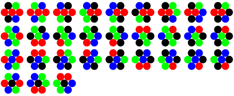
Closure of this calculation can be verified to higher order, but that is not necessary. The numbers indicate thirty total templates, and they can by subdivided by central symbol:
vals = Join[Range[1, 3], {10}];
SortedInds = Cases[Position[templates[[-1]], #], {x_, 2} :> x] & /@ vals;
Length /@ SortedInds
Out[]={9, 9, 9, 3}
The thirty templates are depicted as follows:
DepictTemplate[rule_] := Graphics[{
   Depict[{0, 0, 0}, rule[[2]]],
   MapThread[Depict, {NeighborLocs[{0, 0, 0}, 1], rule[[1]]}]
   }]

GraphicsGrid[ Partition[
  PadRight[Show[DepictTemplate[#], ImageSize -> 75] & /@
    templates[[-1, Flatten[SortedInds]]], 36, Graphics[]], 9]]
As we did with the Penrose tiling, we can compute unique partial completions, and use those to write a set of incontrovertible rules. However, these "obvious" rules are not enough to kick-start growth, and ambiguity can be a problem where branches should terminate. Thus we need to add a few extra rules by inspection, and that allows the derivation to go wrong, briefly.
partials[temp_] :=
 ReplacePart[temp, Alternatives @@ # -> _] & /@
  Subsets[Range[Length[temp]]]

AllPartials =
  Union[Flatten[partials /@ templates[[-1, SortedInds[[#]], 1]],
      1]] & /@ Range[4];

FilteredPartials = Complement[AllPartials[[#]],
     Flatten[AllPartials[[Complement[Range[4], {#}]]] , 1] ] & /@
   Range[4];

Subsets[Range[4], {2}] /. {x_, y_} :>
  Intersection[FilteredPartials[[x]], FilteredPartials[[y]]]

Out[]= {{}, {}, {}, {}, {}, {}}

DefiniteRules =
  Map[Alternatives @@ FilteredPartials[[#]] -> vals[[#]] &, Range[4]];

GetTurnOns[data_] := Select[
  NeighborVals[data, #[[1]] ] -> #[[2]] & /@ data,
  MemberQ[#[[1]], data[[1, 2]] ] &]

OnRules = Join[ Flatten[
    Function[{val}, Union[Flatten[
        GetTurnOns[{T[{0, 0, 0}, val], #}] & /@ DeleteCases[
            DeleteCases[Flatten[T[{0, 0, 0}, val] /. InflateRep],
           T[_, 10]], T[{0, 0, 0}, _]]]]] /@ vals[[1 ;; 3]], 1]];

TermRules = Join[
   RotateRight[{Mod[1 - #, 3] + 1, Mod[3 - #, 3] + 1,
        0 | Mod[2 - #, 3] + 1, 0, 0, 0 | Mod[2 - #, 3] + 1}, # -
        1] -> 10 & /@ Range[0, 5]   ];

AllRules = Join[OnRules, DefiniteRules, TermRules];

State0 = {{T[{0, 0, 0}, 1]}, {}};

Iterate[state_] := With[{newVerts = Complement[
     Flatten[NeighborLocs[#, 1] & /@ state[[1, All, 1]], 1],
     Flatten[state[[All, All, 1]], 1]]},
  Sow[NeighborVals[Flatten[state], #] & /@ newVerts];
  Flatten /@ {MapThread[
     If[IntegerQ[#2], T[#1, #2], {}] &, {newVerts,
      ReplaceAll[NeighborVals[Flatten[state], #],
         AllRules] & /@ newVerts}], state}]

Graphics[Flatten[Nest[Iterate, State0, 15]] /. T -> Depict]
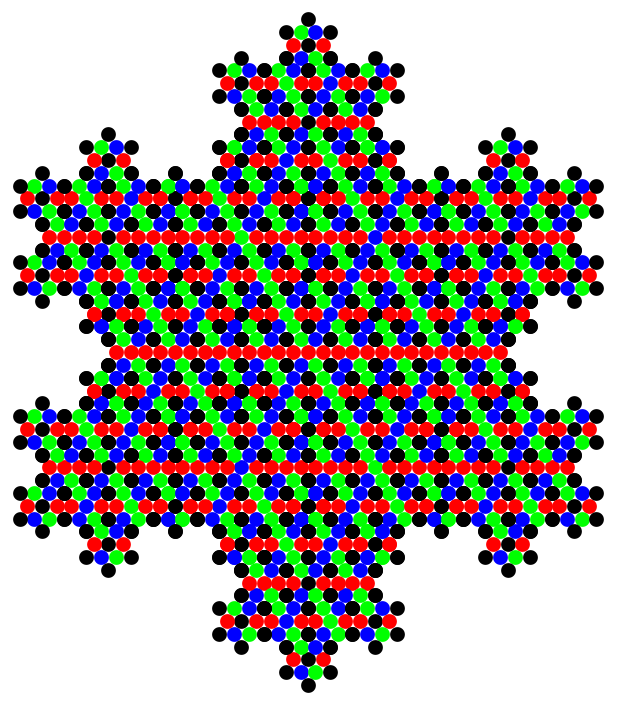
Looking closely we see that periodic patterns are forming in the sextants between principal branches, not what we want. The problem is with termination conditions, which rightly depend on a lookback function through arbitrary many generations. However, the lookback is line-of-sight, so it turns out to be easy to hack by adding three mirror colors. Mirror colors act essentially like the originals, but they are always rooted on black. The modified rules are as follows:
SplitRGB[primary_, secondary_] :=
 Flatten[Function[{a, b}, Select[FilteredPartials[[primary]],
       And[IntegerQ[#[[a]]], IntegerQ[#[[b]]],
         Count[#, _Integer] == 2, MemberQ[#[[{a, b}]], 10]] &]
      ] @@ # & /@ secondary, 1]

DarkMirrorSignals = MapThread[SplitRGB, {{1, 2, 3}, {
     {{1, 2}, {4, 5}, {3, 4}, {1, 6}},
     {{3, 4}, {1, 6}, {2, 3}, {5, 6}},
     {{2, 3}, {5, 6}, {1, 2}, {4, 5}}}}];

FilteredPartials2 = Join[ReplaceAll[
      Complement[#, Flatten[DarkMirrorSignals, 1]],
      {1 -> 1 | -1, 2 -> 2 | -2, 3 -> 3 | -3}
      ] & /@ FilteredPartials, DarkMirrorSignals];

Length /@ FilteredPartials2

Out[]= {278, 278, 278, 108, 8, 8, 8}

Subsets[Range[7], {2}] /. {x_, y_} :>
  Intersection[FilteredPartials2[[x]], FilteredPartials2[[y]]]

Out[]= {{}, {}, {}, {}, {}, {}, {}, {}, {}, {},
{}, {}, {}, {}, {}, {}, {}, {}, {}, {}, {}}

vals = {1, 2, 3, 10, -1, -2, -3};

DefiniteRules2 =
  Map[Alternatives @@ FilteredPartials2[[#]] -> vals[[#]] &, Range[7]];

TermRules2 = Join[
   RotateRight[{Mod[1 - #, 3] + 1, Mod[3 - #, 3] + 1,
        0 | Mod[2 - #, 3] + 1, 0, 0, 0 | Mod[2 - #, 3] + 1}, # -
        1] -> 10 & /@ Range[0, 5],
    RotateRight[{Mod[1 - #, 3] + 1, -(Mod[3 - #, 3] + 1),
        0 | Mod[2 - #, 3] + 1, 0, 0, 0 | Mod[2 - #, 3] + 1}, # -
        1] -> (Mod[2 - #, 3] + 1) & /@ Range[0, 5],
   RotateRight[{-(Mod[1 - #, 3] + 1), Mod[3 - #, 3] + 1,
        0 | Mod[2 - #, 3] + 1, 0, 0, 0 | Mod[2 - #, 3] + 1}, # -
        1] -> (Mod[2 - #, 3] + 1) & /@ Range[0, 5]];

AllRules = Join[OnRules, ReplaceAll[OnRules, {x_Integer :> -x}],
   DefiniteRules2, TermRules2];
Now that we have new AllRules, we can try again:
Graphics[Flatten[Nest[Iterate, State0, 15]] /. T -> Depict]
This looks correct but we had better check by projecting out dark mirror signals, and checking the complement with the inflation output:
AbsoluteTiming[GrowthData54 = NestList[Iterate, State0, 54];]
Out[]= {49.829, Null}

AbsoluteTiming[ InflateData = Union[Flatten[
     T[{0, 0, 0}, 1] /. InflateRep /. InflateRep /. InflateRep /.
       InflateRep /. InflateRep]];]
Out[]= {3.52314, Null}

Complement[ Flatten[GrowthData54[[-1]]] /. T[x_, y_] :> T[x, Abs[y]], InflateData]
Out[]= {}
This check holds to time $81$, and it should probably hold to infinity (but slightly more testing would be nice to improve confidence). The Ulam Structure can be shown by calculating a few integer growth sequences:
Length[#[[1]]] & /@ GrowthData
%[[2 ;; -1]]/6
Flatten[Position[%, 3]]
Differences[%]

Out[]={1, 6, 12, 18, 18, 36, 36, 30, 60, 54, 18, 42, 66, 66, 132, 108, 84,
132, 108, 30, 72, 114, 114, 228, 180, 138, 204, 162, 18, 42, 66, 66,
138, 138, 114, 234, 210, 66, 162, 258, 258, 516, 396, 300, 420, 324,
84, 198, 306, 324, 564, 396, 300, 420, 324, 30, 72, 114, 114, 240,
240, 198, 408, 366, 114, 282, 450, 450, 900, 684, 516, 708, 540, 138,
324, 498, 534, 900, 612, 462, 636, 486, 18}

Out[]={1, 2, 3, 3, 6, 6, 5, 10, 9, 3, 7, 11, 11, 22, 18, 14, 22, 18, 5, 12,
19, 19, 38, 30, 23, 34, 27, 3, 7, 11, 11, 23, 23, 19, 39, 35, 11, 27,
43, 43, 86, 66, 50, 70, 54, 14, 33, 51, 54, 94, 66, 50, 70, 54, 5,
12, 19, 19, 40, 40, 33, 68, 61, 19, 47, 75, 75, 150, 114, 86, 118,
90, 23, 54, 83, 89, 150, 102, 77, 106, 81, 3}

Out[]={3, 4, 10, 28, 82}

Out[]={1, 6, 18, 54}
That is, the growth function returns log-periodically, by a factor $3$, to local minimum growth of turning on only $6 \times 3$ vertices (at hexagonal corners). This is very similar to what we have seen previously. We will update previous threads with counting sequences soon. These are all rigorous, and probably none of them are already in OEIS, assuming originality!
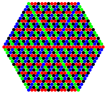
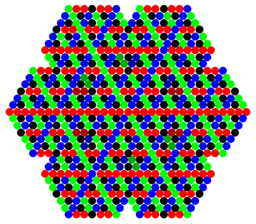
Now we can compare intermediary growth of whole hex and half hex:
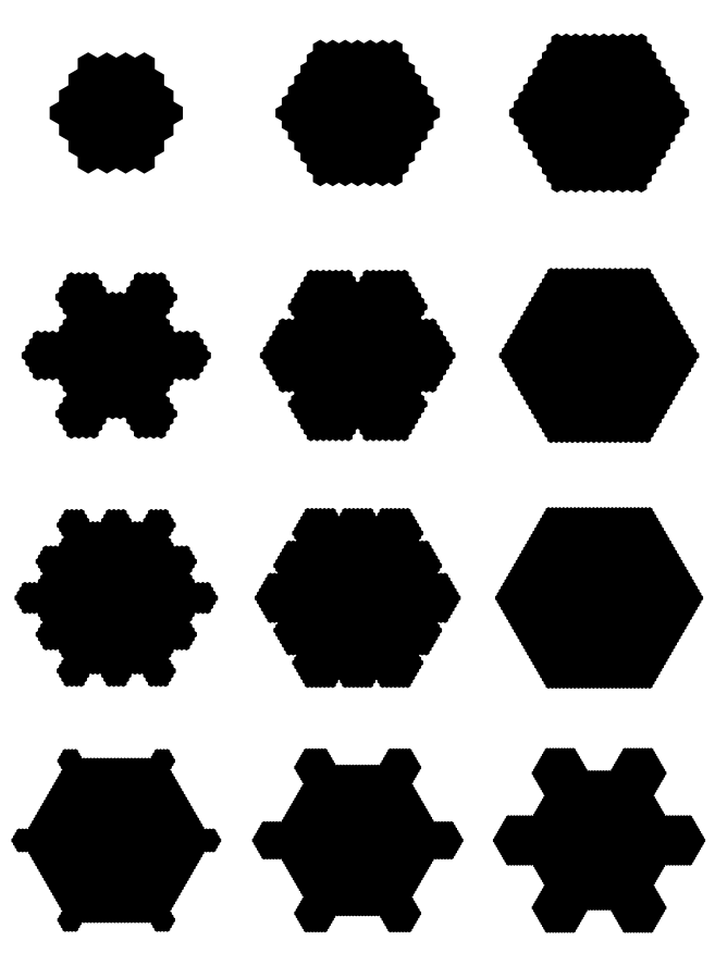
Whole Hex
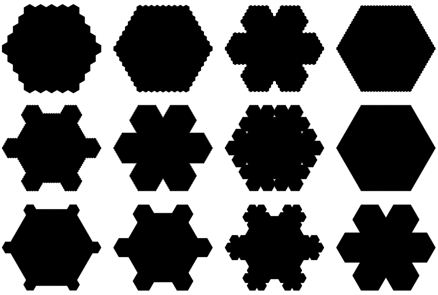
Half Hex
Relative dimensions are different in either model, so we might ultimately find that some plate-like snowflakes look more like patterns produced by one system or the other. If we look closely at whole hex growth, we sometimes see growth forming from a lone black vertex on an otherwise dead edge. This is unnatural relative to growth only from corners, so we expect half-hex to be a better simple model. This expectation does not preclude the possibility that whole hex functions will sometimes fit the data better. It would be interesting to do some data calculations and see what actually happens, but this project we leave for the future.


