Everyone knows, says Carnot, that heat can produce motion. This translation from the late 1800s can produce..the vast movements which take place on the Earth, the ascension of clouds, the meteors part, which man has employed thus but a small portion. The weak censorship hypothesis, posited by Roger Penrose in 1969, suggests that singularities arising from gravitational collapse are..generally concealed within these event horizons, which renders them invisible from the rest of spacetime. The rest of us..have some research that aims to explore the prevalence and robustness of naked singularities. So when you apply several approaches that utilize the discrete nature of spacetime modeled by the Wolfram framework, this is what you get:
torusRegion =
  TransformedRegion[
   DiscretizeRegion[
    ParametricRegion[{(2 + Cos[v]) Cos[u], (2 + Cos[v]) Sin[u],
      Sin[v]}, {{u, 0, 2 Pi}, {v, 0, 2 Pi}}]],
   ScalingTransform[{1, 1, 1}]];
moebiusStripRegion =
  TransformedRegion[
   DiscretizeRegion[
    ParametricRegion[{(1 + v Cos[u/2]) Cos[u], (1 + v Cos[u/2]) Sin[
        u], v Sin[u/2]}, {{u, 0, 2 Pi}, {v, -0.5, 0.5}}]],
   ScalingTransform[{1, 1, 1}]];
coneRegion =
  TransformedRegion[
   DiscretizeRegion[
    ParametricRegion[{u Cos[v], u Sin[v],
      u}, {{u, 0.2, 3}, {v, 0, 2 Pi}}]],
   ScalingTransform[{1, 1, 1}]];
funnelRegion =
  TransformedRegion[
   DiscretizeRegion[
    ParametricRegion[{(2 - u) Cos[v], (2 - u) Sin[v],
      u}, {{u, 0.2, 2}, {v, 0, 2 Pi}}]],
   ScalingTransform[{1, 1, 1}]];
spaceRegionNew = RegionUnion[coneRegion, funnelRegion];
rCone = DiscretizeRegion[
   ParametricRegion[{u Cos[v], u Sin[v],
     u}, {{u, 0.6, 2}, {v, 0, 2 Pi}}]];
hyperbolicParaboloid =
  ParametricRegion[{u, v, u^2 - v^2}, {{u, -1, 1}, {v, -1, 1}}];
spaceRegion =
  RegionUnion[DiscretizeRegion[rCone],
   DiscretizeRegion[hyperbolicParaboloid]];
rTwistedTorus =
  DiscretizeRegion[
   ParametricRegion[{(2 + Cos[u]) Cos[v], (2 + Cos[u]) Sin[v],
     Sin[u] + 0.5 Sin[2 v]}, {{u, 0, 2 Pi}, {v, 0, 2 Pi}}]];
spaceRegion = RegionUnion[rCone, funnelRegion, rTwistedTorus];
r3 = TransformedRegion[
   DiscretizeRegion[
    ParametricRegion[{2 Cos[u]*(2 + Cos[u]) Cos[v],
      2 (2 + Cos[u])*Sin[v], Sin[u]}, {{u, 0, 2 Pi}, {v, 0, 2 Pi}}]],
   ScalingTransform[{1, 1, 2.5}]];
r4 = TransformedRegion[
   DiscretizeRegion[
    ParametricRegion[{(2 + 0.5 + 0.3 Sin[v]) Cos[
        u], (2 + 0.5 + 0.3 Sin[v]) Sin[u],
      2 (v - 2) - 4 + 0.5 Cos[v] + 0.5 Sin[v]}, {{u, 0, 2 Pi}, {v, 2,
       4.5}}]], ScalingTransform[{1, 1, 2.5}]];
spaceRegion = RegionUnion[r3, r4];
generateCausalGraph[region_, numPoints_] :=
  Module[{p, g}, p = RandomPoint[region, numPoints];
   g = TransitiveReductionGraph[
     SimpleGraph[
      Graph[#[[1, 1]] -> #[[2]] & /@
        Catenate[
         With[{v = #},
            Thread[Framed[v] ->
              Select[p, (v[[3]] > #[[
                    3]]) && ((# - v)[[1]]^2 + (# - v)[[
                    2]]^2 + (# - v)[[3]]^2) < 1 &]]] & /@ p],
       VertexStyle -> LightGray]]];
   Graph[g, EdgeStyle -> Black]];
perturb[graph_, method_, hoodVertex_, exteriorVertex_] :=
  Switch[method, "Add Edge",
   Graph[Append[EdgeList[graph],
     DirectedEdge[hoodVertex, exteriorVertex]], VertexStyle -> Orange,
     EdgeStyle -> Black], "Remove Edge",
   Graph[DeleteCases[EdgeList[graph],
     DirectedEdge[hoodVertex, exteriorVertex]], VertexStyle -> Orange,
     EdgeStyle -> Black], "Random Edge",
   With[{newEdge =
      RandomChoice[DirectedEdge @@@ Subsets[VertexList[graph], {2}]]},
     Graph[Append[EdgeList[graph], newEdge], VertexStyle -> Orange,
     EdgeStyle -> Black]], _, graph];
safeRandomChoice[list_] :=
  If[Length[list] > 0, RandomChoice[list], None];
generateAndPerturbGraphs[] :=
 Module[{universeCausalGraphs, methods, hoodVertices,
   exteriorVertices, methodsChosen, universeCausalGraphsPerturbed},
  methods = {"Add Edge", "Remove Edge", "Random Edge"};
  universeCausalGraphs =
   Table[generateCausalGraph[region,
     1500], {region, {torusRegion, moebiusStripRegion, coneRegion,
      funnelRegion, spaceRegionNew, spaceRegion}}];
  methodsChosen =
   RandomChoice[methods, Length[universeCausalGraphs]];
  hoodVertices =
   Table[safeRandomChoice[VertexList[graph]], {graph,
     universeCausalGraphs}];
  exteriorVertices =
   Table[safeRandomChoice[VertexList[graph]], {graph,
     universeCausalGraphs}];
  universeCausalGraphsPerturbed =
   Table[If[
     hoodVertices[[i]] =!= None && exteriorVertices[[i]] =!= None,
     perturb[universeCausalGraphs[[i]], methodsChosen[[i]],
      hoodVertices[[i]], exteriorVertices[[i]]],
     universeCausalGraphs[[i]]], {i, Length[universeCausalGraphs]}];
  universeCausalGraphsPerturbed]
visualizeGraph[graph_, hoodVertex_, exteriorVertex_] :=
  If[hoodVertex =!= None && exteriorVertex =!= None,
   HighlightGraph[
    Graph3D[graph,
     VertexCoordinates -> ((# -> #) & /@ VertexList[graph]),
     VertexSize -> {hoodVertex -> 20, exteriorVertex -> 20},
     VertexStyle -> {hoodVertex -> Red, exteriorVertex -> Blue},
     EdgeStyle -> Black], {Style[
      VertexOutComponent[graph, hoodVertex], Red],
     Style[VertexOutComponent[graph, exteriorVertex], Blue]}],
   Graph3D[graph,
    VertexCoordinates -> ((# -> #) & /@ VertexList[graph]),
    VertexSize -> 5, VertexStyle -> LightGray, EdgeStyle -> Black]];
cylinderHeight = 5;
r1 = DiscretizeRegion[
   ParametricRegion[{Cosh[v]*Cos[u], Cosh[v]*Sin[u],
     2*v}, {{u, -Pi, Pi}, {v, 0, 2}}]];
r2 = DiscretizeRegion[
   ParametricRegion[{Cosh[2]*Cos[u], Cosh[2]*Sin[u],
     cylinderHeight*(v - Sqrt[16 + Cosh[2]^2]) -
      4*(cylinderHeight - 1)}, {{u, -Pi, Pi}, {v,
      Sqrt[16 + Cosh[2]^2], 4 + Sqrt[16 + Cosh[2]^2]}}]];
spaceRegionNew = RegionUnion[r1, r2];
universeCausalGraph1 =
  With[{p = RandomPoint[spaceRegionNew, 6000]},
   With[{g =
      TransitiveReductionGraph[
       SimpleGraph[
        Graph[#[[1, 1]] -> #[[2]] & /@
          Catenate[
           With[{v = #},
              Thread[Framed[v] ->
                Select[p, (v[[3]] > #[[
                    3]]) && ((# - v)[[1]]^2 + (# - v)[[
                    2]]^2 + (# - v)[[3]]^2) < 0.5 &]]] & /@ p],
         VertexStyle ->
          Directive[Hue[0.11, 1, 0.97],
           EdgeForm[{Hue[0.11, 1, 0.97], Opacity[1]}]]]]]},
    Graph[g, EdgeStyle -> Hue[0, 1, 0.56]]]];
findFutureNullInfinity[graphEvolution_] :=
  Module[{initialCausalGraph, finalCausalGraph},
   initialCausalGraph = graphEvolution[[-2]];
   finalCausalGraph = graphEvolution[[-1]];
   Select[
    Complement[VertexList[finalCausalGraph],
     VertexList[initialCausalGraph]],
    VertexOutDegree[finalCausalGraph, #] == 0 &]];
findSingularities[graph_, futureNullInfinityVertex_] :=
  Module[{finalCausalGraph, zeroOutdegreeList},
   zeroOutdegreeList = First /@ Position[VertexOutDegree[graph], 0];
   Complement[zeroOutdegreeList, futureNullInfinityVertex]];
sequences =
  Table[Module[{graphs, hoodVertices, exteriorVertices},
    graphs = generateAndPerturbGraphs[];
    hoodVertices =
     Table[safeRandomChoice[VertexList[graph]], {graph, graphs}];
    exteriorVertices =
     Table[safeRandomChoice[VertexList[graph]], {graph, graphs}];
    Table[
     visualizeGraph[graphs[[i]], hoodVertices[[i]],
      exteriorVertices[[i]]], {i, Length[graphs]}]], {6}];
futureNullInfinityVertexCoord =
  findFutureNullInfinityInSprinkledSpacetime[universeCausalGraph1];
singularitiesCoord =
  findSingularitiesInSprinkledSpacetime[universeCausalGraph1,
   futureNullInfinityVertexCoord];
neighbourhood =
  findNeighbourhood[universeCausalGraph1, singularitiesCoord];
originalShapes = {Graphics3D[torusRegion],
   Graphics3D[moebiusStripRegion], Graphics3D[coneRegion],
   Graphics3D[funnelRegion], Graphics3D[spaceRegionNew],
   Graphics3D[spaceRegion], Graphics3D[rTwistedTorus], Graphics3D[r3],
    Graphics3D[r4]};
{Row[originalShapes], sequences}
The Wolfram Model, that's what gets us working for the Space Research Centre in the Wolfram Research corner. What do you know about the context of general relativity, you could find it on the Wolfram Model's approach to discrete models of spacetime? I'm introducing you to general relativity, I'm going to get these energy-momentum tensors..what with all the equivalence, this article really shows the consistency and covariance. Why I wonder, this has to be within the general relativity context, to balance out with Einstein's field equation hypothesis; I think that getting a little extra space for the energy-momentum tensor, to the geometric properties of spacetime, which are expressed through the Einstein tensor. When I saw Einstein..and presumably if you do an infinite number of batches of the Schwarzchild solution to the Einstein field equations as they are presented they describe the spacetime geometry that exists just by luck around a non-rotating, spherically symmetric mass. It's like the kind of thing you never though could explain the weak cosmic censorship hypothesis. Supposedly as the number of points in a space increases, the occurrence of "fake singularities" diminishes; that's the idea - the artifacts of the discretization process...how does that explain genuine features of spacetime? What if I want to describe them together at the same time? That would make sense, the front-end updates before the analog, the generalization of depth of the solutions to Einstein's equations that are hidden within event horizons, and which cannot be observed from the rest of spacetime..this just shows the depth of these naked singularities which might outperform singularities that are concealed by an event horizon, which just shows how common these are in the Wolfram Rectified Linear Units then, it shows how simple and non-perturbed spacetimes can be diffracted and in this space we might find a more practical approximation of the occurrence of "fake singularities" because as we introduce perturbations in the spacetime, we study their effects on the visibility of singularities, but first, we cant find the weak cosmic censorship hypothesis in the traditional sense. There are no values in discrete spacetime models, that's why further research including a more rigorous mathematical description and extension to the strong cosmic censorship hypothesis, is necessary.
exteriorVerticesN = 50;
inputEvents = Range[exteriorVerticesN];
eventsConnectEvolve[events_, rule_] :=
  Module[{pairs, causalEdges}, pairs = Subsets[events, {2}];
   causalEdges = Select[pairs,
     Which[
       rule == "divisibility",
       Mod[#[[1]], #[[2]]] == 0 || Mod[#[[2]], #[[1]]] == 0,
       rule == "primeConnectivity",
       PrimeQ[#[[1]]] || PrimeQ[#[[2]]] && PrimeQ[#[[1]] + #[[2]]],
       rule == "commonDivisor", GCD[#[[1]], #[[2]]] > 1,
       rule == "difference", Abs[#[[1]] - #[[2]]] < 10,
       rule == "proximity", Abs[#[[1]] - #[[2]]] <= 5, True, False] &];
   DirectedEdge @@@ causalEdges];
generateCausalGraph[inputEvents_, rule_] :=
  Graph[inputEvents, eventsConnectEvolve[inputEvents, rule],
   VertexLabels -> "Name"];
rules = {"divisibility", "primeConnectivity", "commonDivisor",
   "difference", "proximity"};
causalGraphs =
 Table[generateCausalGraph[inputEvents, rule], {rule, rules}]
findSingularities[graph_] :=
  Select[VertexList[graph], VertexOutDegree[graph, #] == 0 &];
findFutureNullInfinity[graph_] :=
  Select[VertexList[graph], VertexInDegree[graph, #] == 0 &];
CausalGraphGeoDesic[graph_, singularities_, futureNullInfinity_] :=
  Module[{layoutOpts = "SpringElectricalEmbedding",
    styleOps = {VertexStyle -> White,
      EdgeStyle -> Directive[GrayLevel[0.7], Opacity[0.7]],
      VertexSize -> Medium, EdgeThickness -> 0.002},
    labelOps = {VertexLabels -> Placed["Name", Center],
      VertexLabelStyle -> Directive[Black, 12]},
    graphOps = {Frame -> True, FrameTicks -> None,
      PlotRangePadding -> 0.1, ImageSize -> Large},
    plotLabelStyle =
     Style["Einsteinian Causal Graph with Singularities (Red) and \
Future Null Infinity (Blue)", 16]},
   Legended[
    HighlightGraph[
     graph, {Style[singularities, Red],
      Style[futureNullInfinity, Blue]},
     GraphLayout -> layoutOpts, styleOps, labelOps, graphOps,
     PlotLabel -> plotLabelStyle],
    SwatchLegend[{Red, Blue}, {"Singularities",
      "Future Null Infinity"}]]];
generateCausalGraphVisualizations[causalGraphs_] :=
  Table[With[{singularities = findSingularities[graph],
     futureNullInfinity = findFutureNullInfinity[graph]},
    CausalGraphGeoDesic[graph, singularities,
     futureNullInfinity]], {graph, causalGraphs}];
causalGraphVisualizations =
  generateCausalGraphVisualizations[causalGraphs];
Okay, the concepts of time dilation are not great, but okay we can perform length contraction and progress from the principles of special relativity to the more general framework of Einstein's theory of gravitation, which explains the concept of spacetime curvature that we are implicitly doing with mass and energy so when you see the experimental tests of general relativity, just remember the overall structure and fate of the universe in just a minute, just remember that the weak cosmic censorship conjecture may be violated in asymptotically flat spaces of five dimensions. Further computational mathematical significance, if you're trying to do these things with a neural net, you're going to have to cascade with handstands to be able to get out of the universal computer and see that singularities may be visible, which would have profound implications for our understanding because fundamentally you're there, in terms of being able to have compositionality. There's no further you can go, quantitative versus qualitative has been formalizing the Wolfram Language from the start in computational terms, which has been the last four centuries of effort, to represent the world in this computational way.
c = 1; G = 1; M = 1;
schwarzschildRadius[mass_] := 2*G*mass/c^2;
edgeAllowedQ[vertex1Coords_, vertex2Coords_, radius_] :=
  Module[{deltaT, deltaS},
   deltaT = vertex2Coords[[1]] - vertex1Coords[[1]];
   deltaS = Norm[vertex2Coords[[2]] - vertex1Coords[[2]]];
   deltaT >= 0 && deltaS <= c*deltaT && deltaS >= radius];
adaptiveTimeStep[currentCoords_, Rs_] :=
  Min[1, 0.1/Norm[currentCoords - {0, Rs}]];
evolveSpacetime[graph_, coords_, steps_, Rs_] :=
  Module[{currentGraph = graph, currentCoords = coords, newEdges,
    newVertices, maxVertex, timeStep},
   Do[timeStep =
     adaptiveTimeStep[currentCoords[[Last@VertexList[currentGraph]]],
      Rs];
    maxVertex = Max[VertexList[currentGraph]];
    newVertices = Range[maxVertex + 1, maxVertex + 3];
    currentCoords =
     Join[currentCoords,
      Table[{i, RandomReal[{0, 3}]}, {i, newVertices}]];
    newEdges =
     Select[Subsets[newVertices, {2}],
      edgeAllowedQ[currentCoords[[First[#]]],
        currentCoords[[Last[#]]], Rs] &];
    currentGraph =
     EdgeAdd[VertexAdd[currentGraph, newVertices],
      UndirectedEdge @@@ newEdges];, {steps}];
   {currentGraph, currentCoords}];
findEventHorizon[graph_] :=
  Module[{eventHorizonVertices},
   eventHorizonVertices =
    Select[VertexList[graph], VertexOutDegree[graph, #] == 0 &];
   eventHorizonVertices];
visualizeCausalGraph[graph_, coords_] :=
  Module[{singularities, eventHorizon},
   singularities = findSingularities[graph];
   eventHorizon = findEventHorizon[graph];
   HighlightGraph[
    graph, {Style[singularities, Red], Style[eventHorizon, Blue]},
    VertexLabels -> "Name", VertexCoordinates -> coords]];
initialCoords = Table[{i, RandomReal[{0, 3}]}, {i, 5}];
initialGraph =
  Graph[Range[5], {}, DirectedEdges -> True,
   VertexCoordinates -> initialCoords, VertexLabels -> "Name"];
Rs = schwarzschildRadius[M];
{evolvedGraph, evolvedCoords} =
  evolveSpacetime[initialGraph, initialCoords, 3, Rs];
visualizedCausalGraph =
  visualizeCausalGraph[evolvedGraph, evolvedCoords];
visualizedCausalGraph
The findings on whether black rings can evolve into naked singularities are significant. If such a transition is possible, it would suggest scenarios where the weak cosmic censorship conjecture might not hold, particularly in higher dimensional spacetimes. We can't assume that the peculiarities and richness of higher-dimensional spacetimes, are a subject of interest in string theory and other areas of theoretical physics. And this sort of teaches you to be an academic, doing middle-school level physics. This really assumes a Gaussian error distribution, the isomorphisms in the gravitational phenomena beyond our familiar four-dimensional spacetime have implications for theories that attempt to unify gravity with quantum mechanics.
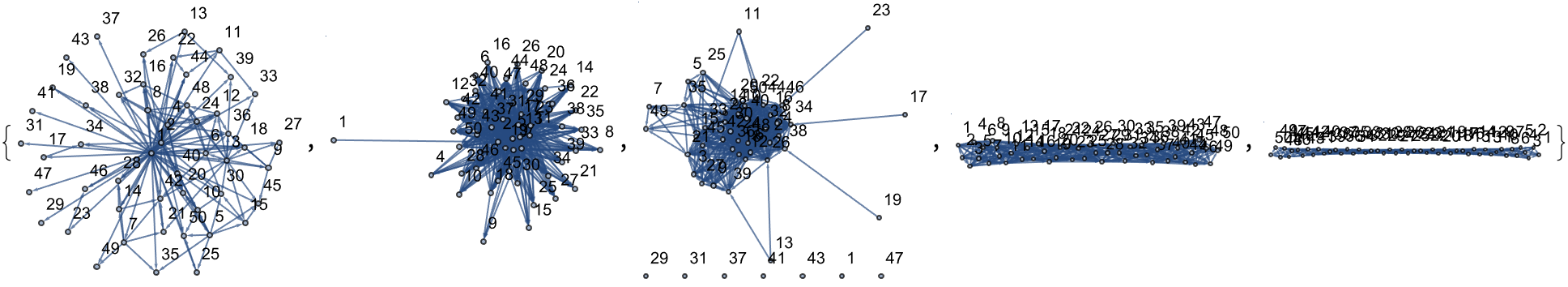
RandomCausalGraph[n_, edgeRatio_] :=
 Module[{edges},
  edges = RandomSample[Tuples[Range[n], 2],
    Round[edgeRatio*n*(n - 1)]];
  Graph[edges, DirectedEdges -> True, VertexLabels -> "Name",
   GraphLayout -> "LayeredDigraphEmbedding"]]
VisualizeCausalGraph[graph_] :=
 HighlightGraph[
  graph, {Style[Subgraph[graph, VertexOutComponent[graph, 1]],
    LightRed], Style[1, Red]}]
mem : FutureNullInfinityVertices[graph_] :=
 mem = Select[VertexList[graph], VertexOutDegree[graph, #] == 0 &]
AnalyzeSingularities[graph_] :=
 Module[{futureNullVertices, singularities, nakedSingularities},
  futureNullVertices = FutureNullInfinityVertices[graph];
  singularities = Complement[futureNullVertices, {1}];
  nakedSingularities =
   Select[singularities, IsNakedSingularity[graph, #] &];
  {"AllSingularities" -> singularities,
   "NakedSingularities" -> nakedSingularities}]
IsNakedSingularity[graph_, singularity_] :=
 Not[AllTrue[VertexInComponent[graph, singularity],
   MemberQ[FutureNullInfinityVertices[graph], #] &]]
n = 50;
edgeRatio = 0.1;
causalGraph = RandomCausalGraph[n, edgeRatio];
visualizedGraph = VisualizeCausalGraph[causalGraph];
singularitiesAnalysis = AnalyzeSingularities[causalGraph];
HighlightGraph[causalGraph,
 MapIndexed[{Style[#1,
     If[MemberQ[singularitiesAnalysis["NakedSingularities"], #1], Red,
       Blue]]} &, singularitiesAnalysis["AllSingularities"]],
 GraphLayout -> "LayeredDigraphEmbedding", VertexLabels -> "Name"]

n = 50;
edgeRatio = 0.1;
causalGraph = RandomCausalGraph[n, edgeRatio];
sinkNodes = FutureNullInfinityVertices[causalGraph];
HighlightGraph[causalGraph, Style[#, Green] & /@ sinkNodes,
 GraphLayout -> "LayeredDigraphEmbedding", VertexLabels -> "Name"]
There are practical things about these thresholds associated with particular things that we can do, consolidating the occurrences of 'naked singularities' not enclosed by an event horizon which, such occurrences twice challenge the understanding of spacetime's behavior under extreme gravitational conditions. Maybe we could say complex numerical simulations evolve the spacetime geometries and study the dynamics of black rings under various conditions..and we could prove..improve in moderation, which is actually quite surprising with regard to the ultimate fate of perturbed black rings. Do they break apart, collapse into black holes, or form naked singularities?
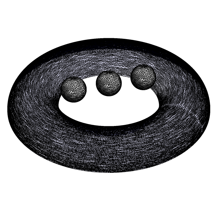
glass = ParametricRegion[{Cos[u]*v, Sin[u]*v,
    u}, {{u, 0, 6 Pi}, {v, 0.8, 1}}];
iceCube1 =
  ParametricRegion[{0.2 Cos[u] + 0.5, 0.2 Sin[u] + 0.5,
    0.2 v}, {{u, 0, 2 Pi}, {v, 0, 2 Pi}}];
iceCube2 =
  TransformedRegion[iceCube1, TranslationTransform[{0.4, 0.4, 1}]];
iceCube3 =
  TransformedRegion[iceCube1, TranslationTransform[{0.8, 0.8, 1.5}]];
discretizedGlass = DiscretizeRegion[glass, MaxCellMeasure -> 0.01];
discretizedIceCube1 =
  DiscretizeRegion[iceCube1, MaxCellMeasure -> 0.01];
discretizedIceCube2 =
  DiscretizeRegion[iceCube2, MaxCellMeasure -> 0.01];
discretizedIceCube3 =
  DiscretizeRegion[iceCube3, MaxCellMeasure -> 0.01];
combinedRegions =
  RegionUnion[discretizedGlass, discretizedIceCube1,
   discretizedIceCube2, discretizedIceCube3];
Graphics3D[{Opacity[0.5, Blue], discretizedGlass, Opacity[0.9, White],
   discretizedIceCube1, Opacity[0.9, White], discretizedIceCube2,
  Opacity[0.9, White], discretizedIceCube3}, Boxed -> False,
 Lighting -> "Neutral"]
There can be only one way to customize our study of black ring instabilities, which can lead to various phenomena such as the break-up of a black ring or its transition into a more stable structure, like a black hole. And that's a very specific way to get us over the weak cosmic censorship conjecture..which is positing that singularities arising from gravitational collapse are always hidden within event horizons..but are they? Are they always invisible to distant observers? I think this hypothesis being fundamental to the predictability of physics beyond an event horizon..a disembodied self-driving car can zoom off but the humans are going to say, who cares? So which direction do you want to drive in? How do humans fit into the world of AIs? Yes, the AIs can provide the naked singularities, the violation of the conjecture that implies the existence of 'naked singularities' that are singularities, that aren't enclosed by an event horizon. You won't get an event horizon.
glass = DiscretizeRegion[
   ParametricRegion[{(3 + Cos[v]) Cos[u], (3 + Cos[v]) Sin[u],
     v}, {{u, 0, 2 Pi}, {v, 0, 4}}],
   MaxCellMeasure -> {"Length" -> 0.2}];
iceCube1 =
  DiscretizeRegion[
   ParametricRegion[{x, y,
     z}, {{x, -0.5, 0.5}, {y, -0.5, 0.5}, {z, -0.5, 0.5}}],
   MaxCellMeasure -> {"Length" -> 0.1}];
iceCube2 =
  DiscretizeRegion[
   ParametricRegion[{x, y,
     z}, {{x, -0.3, 0.3}, {y, -0.3, 0.3}, {z, -0.3, 0.3}}],
   MaxCellMeasure -> {"Length" -> 0.1}];
Graphics3D[{{Opacity[0.1], EdgeForm[], Blue, glass}, {Opacity[1],
   EdgeForm[], White, iceCube1}, {Opacity[1], EdgeForm[], White,
   iceCube2}}, Lighting -> "Neutral", Boxed -> False]

Before all that natural language processing, there's hypergraph rewriting. There is a certain sense in which the propagation of something and making it exist is a self-fulfilling thing to happen. It's an either-or; it's like looking for the output from iFrames, it's like spell-checking the order of priority of the visualizations of the features that we have investigated through computational experiments, and that is actually how we determine how closely the model corresponds to the predictions of general relativity. I want to be able to have a comprehensive, with formatting..be able to navigate through non-traditional black holes like black rings..which are hypothetical objects in higher dimensions (specifically in five dimensions). These are shaped like a torus they have a doughnut shape, and are solutions to the higher-dimensional Einstein field equations which leads to a lot of discordant instabilities which is crucial for understanding the dynamics and end states of these objects.
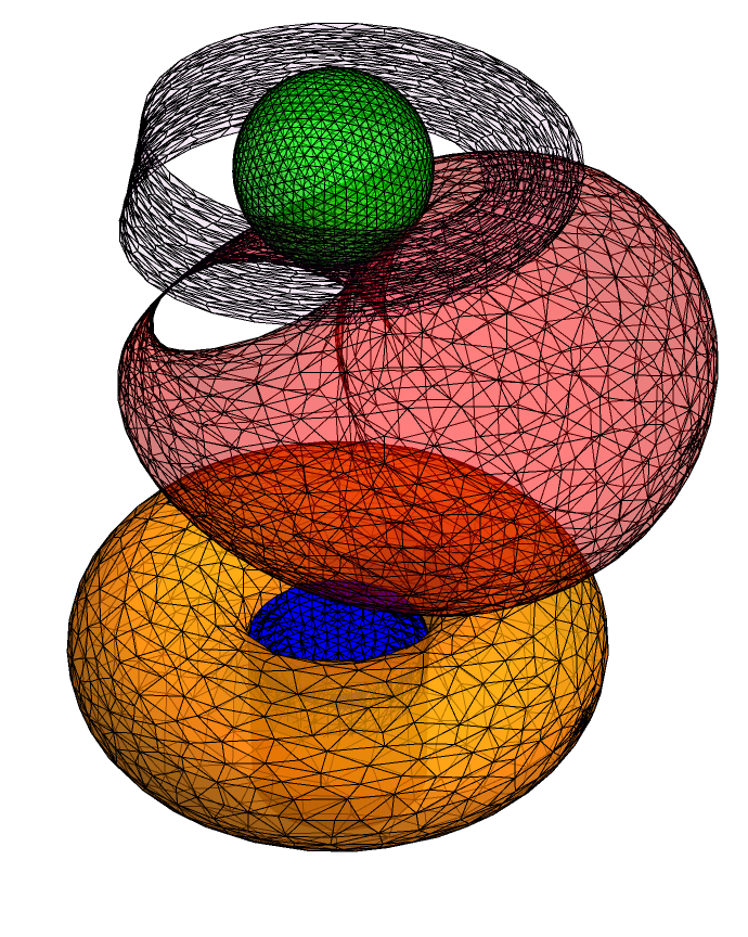
r1 = DiscretizeRegion[
   ParametricRegion[
    {
     (2 + Cos[v])*
      (2 + Cos[u])*
      Cos[v],
     (2 + Cos[v])*
      (2 + Cos[u])*
      Sin[v],
     Sin[u]
     }, {
     {u, 0, 2 Pi},
     {v, 0, 2 Pi}
     }
    ]
   ];
r2 = DiscretizeRegion[
   ParametricRegion[
    {
     (2 + 0.5*Sin[2 u])*
      Cos[u],
     (2 + 0.5*Sin[2 u])*
      Sin[u],
     (1 + 0.5*Sin[2 u] +
         v/(4 (5 - 1))) 5 - 4 (5 - 1)},
    {
     {u, 0, 2 Pi},
     {v, 0, 4 (5 - 1)}
     }
    ]
   ];
r3 = TransformedRegion[
   DiscretizeRegion[
    ParametricRegion[
     {
      2*Cos[u]*(2 + Cos[u])*Cos[v],
      2*(2 + Cos[u])*Sin[v],
      Sin[u]
      },
     {
      {u, 0, 2 Pi},
      {v, 0, 2 Pi}
      }
     ]
    ],
   ScalingTransform[{1, 1, 2.5}]
   ];
r4 = TransformedRegion[
   DiscretizeRegion[
    ParametricRegion[
     {
      (2 + 0.5 + 0.3 Sin[v]) Cos[u],
      (2 + 0.5 + 0.3 Sin[v]) Sin[u],
      2 (v - 2) - 4 + 0.5 Cos[v] + 0.5 Sin[v]
      }, {
      {u, 0, 2 Pi},
      {v, 2, 4.5}
      }
     ]
    ],
   ScalingTransform[{1, 1, 2.5}]
   ];
Graphics3D[{EdgeForm[],
  Lighting -> "Neutral",
  Specularity[White, 10],
  PlotStyle -> Directive[
    Opacity[0.8],
    ColorData[97, "ColorList"][[1]]]
  , r1},
 Boxed -> False,
 ViewPoint -> {0, 0, 5}
 ]
RegionPlot3D[
 r2,
 PlotPoints -> 100,
 MaxRecursion -> 3,
 ColorFunction -> (ColorData["BrightBands", #3] &),
 Boxed -> False,
 Axes -> False,
 Lighting -> "Neutral"
 ]
Graphics3D[{
  EdgeForm[],
  RGBColor[0.8, 0.8, 0.8],
  Lighting -> "Neutral",
  Specularity[White, 10],
  {RGBColor[1, 0.5, 0.5], r4},
  {RGBColor[0.5, 0.5, 1], r3}
  }, Boxed -> False,
 ViewPoint -> {0, 0, 5}
 ]
spaceRegion = RegionUnion[r3, r4];
evolutionLists = {};
universeCausalGraphr1 =
 With[{p = RandomPoint[r1, 1000]},
  With[{g =
     TransitiveReductionGraph[
      SimpleGraph[
       Graph[#[[1, 1]] -> #[[2]] & /@
         Catenate[
          With[{v = #},
             Thread[Framed[v] ->
               Select[p, (v[[3]] > #[[3]]) && ((# - v)[[1]]^2 + (# -
                    v)[[2]]^2 + (# - v)[[3]]^2) < 0.5 &]]] & /@ p],
        VertexStyle ->
         Directive[Hue[0.11, 1, 0.97],
          EdgeForm[{Hue[0.11, 1, 0.97], Opacity[1]}]]]]]},
   Graph[g, EdgeStyle -> Hue[0, 1, 0.56]]]]
universeCausalGraphr2 =
 With[{p = RandomPoint[r2, 1000]},
  With[{g =
     TransitiveReductionGraph[
      SimpleGraph[
       Graph[#[[1, 1]] -> #[[2]] & /@
         Catenate[
          With[{v = #},
             Thread[Framed[v] ->
               Select[p, (v[[3]] > #[[3]]) && ((# - v)[[1]]^2 + (# -
                    v)[[2]]^2 + (# - v)[[3]]^2) < 0.5 &]]] & /@ p],
        VertexStyle ->
         Directive[Hue[0.11, 1, 0.97],
          EdgeForm[{Hue[0.11, 1, 0.97], Opacity[1]}]]]]]},
   Graph[g, EdgeStyle -> Hue[0, 1, 0.56]]]]
universeCausalGraphr3r4 =
 With[{p = RandomPoint[spaceRegion, 1000]},
  With[{g =
     TransitiveReductionGraph[
      SimpleGraph[Graph[#[[1, 1]] -> #[[2]] & /@ Catenate[
          With[{v = #},
             Thread[Framed[v] -> Select[p, (v[[3]] > #[[3]]) && (
                    (# - v)[[1]]^2 +
                    (# - v)[[2]]^2 +
                    (# - v)[[3]]^2
                    ) < 0.5 &]
              ]] & /@ p],
        VertexStyle -> Directive[Hue[0.11, 1, 0.97],
          EdgeForm[{Hue[0.11, 1, 0.97], Opacity[1]}]
          ]]]]},
   Graph[g, EdgeStyle -> Hue[0, 1, 0.56]]]]
AppendTo[evolutionLists, {universeCausalGraph}];
maxEvolutionSteps = 5;
Do[lastCausalGraph = evolutionLists[[-1, -1]];
 newCausalGraph = With[{
    p = VertexList[lastCausalGraph] /. Framed[pt_] :> pt},
   With[{g =
      TransitiveReductionGraph[
       SimpleGraph[Graph[#[[1, 1]] -> #[[2]] & /@ Catenate[
           With[{v = #},
              Thread[Framed[v] -> Select[p,
                 (v[[3]] > #[[3]]) && (
                    (# - v)[[1]]^2 +
                    (# - v)[[2]]^2 +
                    (# - v)[[3]]^2
                    ) < 0.5 &]]] & /@ p],
         VertexStyle -> Directive[
           Hue[0.11, 1, 0.97],
           EdgeForm[{
             Hue[0.11, 1, 0.97],
             Opacity[1]}]
           ]]]]},
    Graph[g, EdgeStyle -> Hue[0, 1, 0.56]]]];
 AppendTo[evolutionLists, {newCausalGraph}],
 {i, 1, maxEvolutionSteps - 1}]
visualize[evolutionLists[[4, -1]], {1, 1}]
Options[causalGraphPlot] = {VertexSize -> 0.05,
   EdgeStyle -> Arrowheads[0.02]};
causalGraphPlot[causalGraph_, options : OptionsPattern[]] := Module[
  {edges, coords, vertices},
  edges = EdgeList[causalGraph];
  coords = PropertyValue[causalGraph, VertexCoordinates];
  vertices = PropertyValue[causalGraph, VertexList];
  Graph[vertices,
   edges,
   VertexCoordinates -> coords,
   VertexSize -> OptionValue[VertexSize],
   EdgeStyle -> OptionValue[EdgeStyle],
   ImageSize -> Medium,
   PlotRangePadding -> Scaled[0.1],
   ImagePadding -> 20,
   GraphLayout -> {"LayeredDigraphEmbedding", "Orientation" -> Top}
   ]]
causalGraphPlot[evolutionLists[[4, -1]]]
causalGraphPlot[evolutionLists[[4, -1]], VertexSize -> 0.03,
 EdgeStyle -> {Black, Arrowheads[0.01]}]
Because we have @James Boyd who participates in everything from differential equations to quantum computing enthusiastically. The Wolfram Model makes recreating features of spacetime a breeze - whether it's black holes or event horizons, using discrete points and connections, we can always find a feature to investigate through computational experiments to demonstrate and determine how closely the model corresponds, because I don't know..to the predictions of general relativity. Causal graphs are complex networks that evolve according to simple computational rules and are hypothesized to mimic the structure and dynamics of spacetime. It's so hard to go outside of one's current human purpose, the things that have sort of been bashed into us..to go to the abstract purpose.
@James Boyd is also that librarian with the periodic table and yes, we see that part of the discrete model of spacetime. Computational models like the Wolfram Model can contribute to our understanding of complex physical theories. It's all on us who have got these new avenues for research and throw up potentially novel interpretations of physical laws and principles as they may apply to computational systems. Computational experiments, that is that determine how closely the model corresponds to the predictions that are of general relativity.
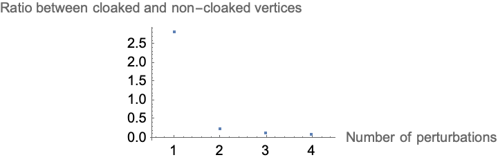
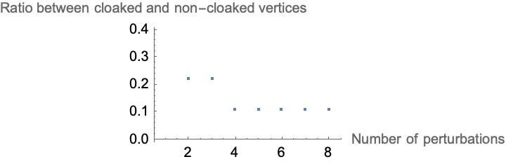
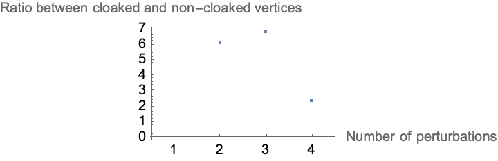
We are able to make it work because the more perturbations we introduce, the more vertices from the singularity neighborhood go outside of the event horizon to null infinity. It deals with the global nature of spacetime and the strong cosmic censorship hypothesis that we must explore, is a more comprehensive version of the weak hypothesis.
Your hypothesis is so robust in discrete models of spacetime. Have a biological organism that has the same memories that can remember from 300 years or so on, how much of that will be sort of owned by these visualizations of the causal graphs..singularities are red, event horizons are blue, and future null infinity is green. There is a direct correlation between the number of perturbations and the ratio of cloaked to non-cloaked events. The weak cosmic censorship hypothesis is not entirely robust in the Wolfram Model.
It suggests further work, we need to do an investigation of the strong censorship hypothesis. Something which grows like us, but doesn't go out of control like that..which indicates a grounding established physics literature. Welcome to Stephen Wolfram's works on relativity, gravitation, and cosmology..we didn't mean for people to like you more than me..then I could say whatever I want related to the weak cosmic censorship conjecture. Have a protractor! I think that I might present a detailed methodology for simulating and analyzing various spacetime configurations. But we won't stop violating the Schwarzschild spacetime solution to Einstein's field equations...but it's okay because the gravitational field is outside a spherical, non-rotating mass such as a star or a black hole.
Many thanks to @Yorick Zeschke who comes from afar making it a positive learning environment. I would also like to thank my State Farm agent, can you turn the clock back within an organism..this ice cube is getting too big for the bottle. We need some image-based functions like findFutureNullInfinity or findSingularities, inEventHorizonQ and findAntichain, and we have various neighborhood and visualization functions and it's like, really? It gets it accurate and for the machine learning classifier..what's going on? What's going on is that there are gradual changes in facial structure, geometrically, the plates of the skull fuse and so on, and over the course of many decades I'm flipping out my astrolabe, I'm coordinatizing the mathematical description of the phenomena observed with the stars, I'm fully understanding the energy-momenta tensor in greater depth and its implications for the validity of the censorship hypotheses in the Wolfram Model.
This decrease in the number of fake naked singularities with an increase in the number of "sprinkled points" in the Wolfram Model..space is just a large collection of discrete points connected by patterns of connections, sprinkled so we can see future null infinity, the event horizons, the singularities. But they might change - your approach to life might be different depending on hormone levels that has little to do with the brain as such; to maintain the usness as it; when it comes to maintaining the package, that's the question is can you do that. How will one increase longevity? To illustrate the structural data impact of increasing the number of points sprinkled across the space on the number of "fake naked singularities"..shows a clear decrease. We don't want to break the character of the weak censorship hypothesis so that we can apply these visualizations, which may not be as robust in discrete models of spacetime. The Wolfram Model, indicates that small perturbations can have a significant impact on the structure of spacetime.
With the energy-momenta tensor, it is only natural. Our species has built those things, but we get to see a new feature of the universe when we do that and one might imagine that guess what - if only, we had managed to tap into the gravitational wave internet, then we would discover the aliens. And in some sense those things are true, like that or this, inefficient decrease in discussion on how the Wolfram Model simulates spacetime using discrete points and connections..there's a direct analog and it's pretty close to the continuous fabric of space-time in general relativity. In the same way that we're not going to be needing the observed singularities, which may be artifacts due to the limitations of a discretized spacetime rather than actual physical phenomena...this ties into the finite density of points in the sprinkling process, which relates to the Poisson distribution used in the model. There's this whole graveyard of discretized spacetime in which perturbing different regions of spacetime - perturbations at the top of a light cone creating fewer observable "naked" singularities compared to perturbations from the bottom, which is in line with the behavior of the emes as they float about at the top of the light cone..the theoretical predictions and experimental observations.
Map[
 Graph3D[#,
   VertexCoordinates -> VertexList[#],
   VertexSize -> 20] &,
 {
  universeCausalGraphr1,
  universeCausalGraphr2,
  universeCausalGraphr3r4
  }
 ]
That's nice, Nikola..like playing those sounds generated with Wolfram Language. @Chase Marangu Because we came down to the sunset at 12:30am because it's the polar sunset with the 2 hour long nights, that was our Claire de Lune. Remember to run these perturbations..how am I supposed to know about the continuous fabric of spacetime in general relativity? Because I want to introduce perturbations and affect the visibility of singularities, with a higher number of perturbations increasing the ratio of visible (cloaked) to non-visible (non-cloaked) events..and thereby, we have challenged the weak cosmic censorship hypothesis within the discrete spacetime model.
graphNum = graphAndSingularityNumbers[[i, 1]];
singularityNum = graphAndSingularityNumbers[[i, 2, 1]];
graph = evolutionLists[[graphNum]][[-1]];
futureNullInfinity =
  findFutureNullInfinity[evolutionLists[[graphNum]]];
vertexLengths = AssociationMap[
   Length[
     VertexOutComponent[graph, #]] &,
   VertexList[graph]
   ];
highlightedGraph = HighlightGraph[graph,
   {Style[n1[[1]], Blue],
    Style[singularityNum, Red],
    Style[futureNullInfinity, Green]}];
vertexStyles = {n1[[1]] -> Blue,
   singularityNum -> Red,
   futureNullInfinity -> Green};
edgeStyles = {DirectedEdge[n1[[1]],
     singularityNum] -> Directive[Red, Thick, Arrowheads[Large]],
   DirectedEdge[n1[[1]], futureNullInfinity] ->
    Directive[Green, Dashed, Arrowheads[Large]]};
Graph[highlightedGraph,
 VertexLabels -> Normal[vertexLengths],
 VertexSize -> {n1[[1]] -> 0.3, singularityNum -> 0.3,
   futureNullInfinity -> 0.3},
 VertexStyle -> vertexStyles,
 EdgeStyle -> edgeStyles,
 ImageSize -> Medium,
 PlotRangePadding -> Scaled[0.1],
 ImagePadding -> 20]
Anyway it's been a fun roller coaster following the @Nikola Bukowiecka path, woo hoo! The fundamental problem is if we could keep a beam of light perfectly columnated..it's inevitable that it would spread out..we have to put an incredible power into it, so we'll still get something reasonable back...you send an, analysis of non-perturbed Schwarzschild spacetime created from the distribution of points, the "sprinkling" technique that casually makes the behavior of singularities count! Having the foundational technique, which you've got it or you don't, without "sprinkling" we would be unable to discretize and discuss the "free" use of the Wolfram Model to visualize and analyze Einstein's field equations. The only thing that distinguishes the eddies of the Riemann curvature tensor from the principles of equivalence is the examination of Schwarzschild spacetime with spacetime perturbations introduced ...which typically involves tensor calculus and differential geometry, similar to the concept of Maxwell's demon.
glass = DiscretizeRegion[
   ParametricRegion[{Sin[v] Cos[u], Sin[v] Sin[u],
     v}, {{u, 0, 2 Pi}, {v, 0, 4}}],
   MaxCellMeasure -> {"Length" -> 0.1}];
iceCube1 =
  DiscretizeRegion[
   ParametricRegion[{0.5 Sin[v] Cos[u], 0.5 Sin[v] Sin[u],
     0.5 Cos[v] + 3}, {{u, 0, 2 Pi}, {v, 0, Pi}}],
   MaxCellMeasure -> {"Length" -> 0.1}];
iceCube2 =
  TransformedRegion[iceCube1, TranslationTransform[{1, 1, 0}]];
iceCube3 =
  TransformedRegion[iceCube1, TranslationTransform[{-1, -1, 0}]];
combinedRegion = RegionUnion[glass, iceCube1, iceCube2, iceCube3];
Graphics3D[{Opacity[0.1], Blue, glass, Opacity[1], White, iceCube1,
  iceCube2, iceCube3}, Lighting -> "Neutral", Boxed -> False,
 Axes -> False]
It still feels cooler if there's a friendly human who went there with a robotic probe, and this is how Qooley got started. We tested out algorithms for calculating future null infinity, event horizons, singularities, and their neighborhoods. On these graphs, an "end" could be a vertex with no outgoing edges, which is also known as a sink. Since these graphs represent causal events, then these sinks could represent final events that are not the cause of any other event in the graph programmatically ...if only, the empirical investigation of spacetime generated by simple, non-perturbed, non-trivial signature rules, could be metrically visualized - then the tensor's components can show how spacetime is curved differently around the Schwarzschild radius.
glass = DiscretizeRegion[
   ParametricRegion[{(3 + Cos[v]) Cos[u], (3 + Cos[v]) Sin[u],
     v}, {{u, 0, 2 Pi}, {v, -5, 0}}], MaxCellMeasure -> 0.1];
iceCube =
  DiscretizeRegion[
   ParametricRegion[{x, y,
     z}, {{x, -0.5, 0.5}, {y, -0.5, 0.5}, {z, -0.5, 0.5}}],
   MaxCellMeasure -> 0.01];
iceCubes =
  Table[TransformedRegion[iceCube,
    TranslationTransform[{RandomReal[{-2, 2}], RandomReal[{-2, 2}],
      RandomReal[{-4, -1}]}]], {n, 1, 5}];
combinedRegion = RegionUnion[glass, Sequence @@ iceCubes];
Graphics3D[{{Opacity[0.1], Blue, glass}, {Opacity[1], White,
   EdgeForm[Black], iceCubes}}, Lighting -> "Neutral", Boxed -> False]
I didn't want to date myself so I left the graphs all on here just to accentuate what I got from elsewhere; there's neither beginnings nor ends to the Wheel of Time. But it was a beginning. Because I don't know what the subject is...I wish that we would change how we describe concepts from general relativity. You could sort of dehumanize ...how important is it to see with your eyes, Alpha Centura? If you get photons in there..you'd be jumping to conclusions just not in the conventional sense. That's what the weak cosmic censorship hypothesis is really describing; the photon gets multiplied by a future version of itself and the singularities arising from gravitational collapse are hidden behind event horizons and thus cannot be observed from the rest of spacetime. The weak cosmic censorship hypothesis suggests that and if they are, visible singularities, that are referred to as "naked", do not exist in nature.
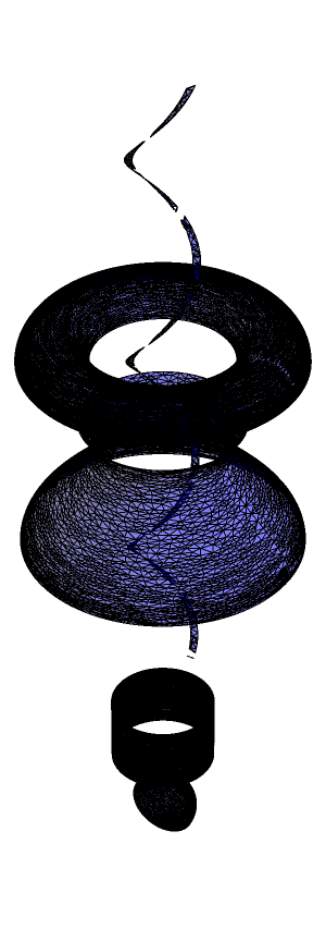
cylinder = Cylinder[{{0, 0, 0}, {0, 0, 2}}, 1];
torus = ParametricRegion[{(2 + Cos[v]) Cos[u], (2 + Cos[v]) Sin[u],
    Sin[v]}, {{u, 0, 2 Pi}, {v, 0, 2 Pi}}];
sphere = Sphere[{0, 0, 4}, 1];
kleinBottle =
  ParametricRegion[{(2 + (1 + Cos[v]) Cos[u]) Cos[
      v], (2 + (1 + Cos[v]) Cos[u]) Sin[v], (1 + Cos[v]) Sin[u]}, {{u,
      0, 2 Pi}, {v, 0, 2 Pi}}];
mobiusStrip =
  ParametricRegion[{(2 + v Cos[u/2]) Cos[u], (2 + v Cos[u/2]) Sin[u],
    v Sin[u/2]}, {{u, 0, 2 Pi}, {v, -0.5, 0.5}}];
discretizedCylinder =
  DiscretizeRegion[cylinder, MaxCellMeasure -> 0.1];
discretizedTorus = DiscretizeRegion[torus, MaxCellMeasure -> 0.1];
discretizedSphere = DiscretizeRegion[sphere, MaxCellMeasure -> 0.1];
discretizedKleinBottle =
  DiscretizeRegion[kleinBottle, MaxCellMeasure -> 0.1];
discretizedMobiusStrip =
  DiscretizeRegion[mobiusStrip, MaxCellMeasure -> 0.1];
transformedTorus =
  TransformedRegion[discretizedTorus, TranslationTransform[{0, 0, 2}]];
transformedSphere =
  TransformedRegion[discretizedSphere,
   TranslationTransform[{0, 0, 4}]];
transformedKleinBottle =
  TransformedRegion[discretizedKleinBottle,
   TranslationTransform[{0, 0, 6}]];
transformedMobiusStrip =
  TransformedRegion[discretizedMobiusStrip,
   TranslationTransform[{0, 0, 8}]];
combinedRegion =
  RegionUnion[discretizedCylinder, transformedTorus,
   transformedSphere, transformedKleinBottle,
   transformedMobiusStrip];
Graphics3D[{Opacity[0.9], Blue, discretizedCylinder, Opacity[0.7],
  Orange, transformedTorus, Opacity[0.5], Green, transformedSphere,
  Opacity[0.3], Red, transformedKleinBottle, Opacity[0.1], Purple,
  transformedMobiusStrip}, Boxed -> False, Lighting -> "Neutral"]
Causal sets - an approach to quantum gravity where spacetime is discrete - can be integrated into the Wolfram Model. And I do, I always think about Gorard's work more than I think about the mathematical structures, that consist of elements and relations that represent the causal ordering of spacetime events. It only makes the rules within this model look more simple, when we see these complex structures that have properties..like for instance when Fermat's last theorem was proved, the chap who proved it, and I asked him and he said I just sort of did it using common mathematics of the time, to say can you just drill mechanically from certain axioms and there are efforts in modern times to make proof assistance. But when you see how these theories of quantum gravity emerge, the computational mechanism ...for the emergence of spacetime ...because that's the kind of conversation that we're going to be having.
region1 =
  ParametricRegion[{Cos[u]*Sin[v], Sin[u]*Sin[v],
    Cos[v]}, {{u, 0, Pi}, {v, 0, Pi}}];
region2 =
  ParametricRegion[{1.5 Cos[u], 1.5 Sin[u],
    v}, {{u, 0, 2 Pi}, {v, -1, 1}}];
region3 =
  ParametricRegion[{Cos[u]*v, Sin[u]*v,
    u}, {{u, 0, 6 Pi}, {v, 0.8, 1}}];
region4 =
  ParametricRegion[{(3 + Cos[v]) Cos[u], (3 + Cos[v]) Sin[u],
    v}, {{u, 0, 2 Pi}, {v, 0, 4}}];
region5 =
  ParametricRegion[{(3 + Cos[v])*Cos[u], (3 + Cos[v])*Sin[u],
    2 + Sin[v]}, {{u, 0, 2 Pi}, {v, 0, Pi}}];
discreteRegions =
  DiscretizeRegion /@ {region1, region2, region3, region4, region5};
transforms = {Identity, TranslationTransform[{0, 0, 3}],
   TranslationTransform[{0, 0, 6}], TranslationTransform[{0, 0, 10}],
   TranslationTransform[{0, 0, 14}]};
combinedRegion =
  RegionUnion @@
   MapThread[TransformedRegion, {discreteRegions, transforms}];
Graphics3D[{Blue, Opacity[0.5], combinedRegion}, Boxed -> False,
 Axes -> False]
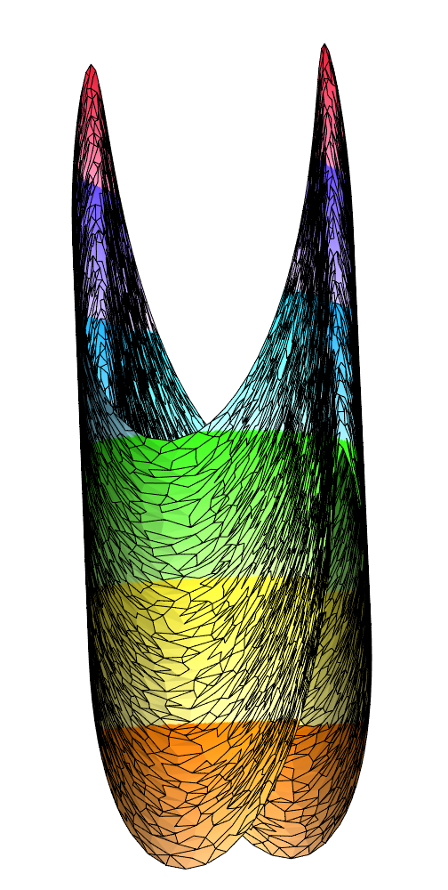
In a sense, the event horizon can develop a pattern of bulges connected by ever-thinning necks. If a civilization wrote down all their discoveries, but the civilization was exterminated..I'm just going to pull out my..what was it? That's right, I pull my astrolabe right out of my pocket as always and I just get into deep philosophy, questions about the purpose of the universe..meaningfully can't be said to have one...we're trying to raise the conditions under which singularities might be visible, which would have profound implications for how we locally diffuse singularities in all directions to build an event handler for handling singularities in numerical general relativity. I think I finally understand how the evolution of the Wolfram Model can be done in a single pass via stochastic gradient descent sampling of the computational models that Wolfram introduces, he introduces hypergraphs that evolve by simple rules. I was going to cite the thing, the Physics Project at the beginning because that's what we're hoping to use throughout our exploration of quantum gravity where spacetime is discrete, and I didn't want to admit that actually, the evolution of simple rules within the Wolfram Model gives rise to the complex structures that have all these properties and show the computational mechanism for the emergence of spacetime from discrete, non-spatial, and non-temporal elements which is what allows us to perform ever since the 1700s, it allows us to visualize a lot of multi-dimensional space via the computational mechanism of linear algebra, or more generally the algebra that is required for this massive computational paradigm of the Wolfram Model. And that was the discovery of how Euclid's axioms are sort of this bubble out there that is not related as such to physical reality.
discretizeWithOpts[region_, opts___] := DiscretizeRegion[region, opts];
cylindricalRegion =
  ParametricRegion[{Cos[\[Theta]], Sin[\[Theta]],
    z}, {{\[Theta], 0, 2 \[Pi]}, {z, 0, 1}}];
cuboidalRegion1 =
  ParametricRegion[{x, y, z}, {{x, -1, 1}, {y, -1, 1}, {z, -1, 1}}];
cuboidalRegion2 =
  ParametricRegion[{x, y,
    z}, {{x, -0.5, 0.5}, {y, -0.5, 0.5}, {z, -0.5, 0.5}}];
sphericalRegion =
  ParametricRegion[{Sin[v] Cos[u], Sin[v] Sin[u],
    Cos[v]}, {{u, 0, 2 \[Pi]}, {v, 0, \[Pi]}}];
dCylindrical =
  discretizeWithOpts[cylindricalRegion,
   MaxCellMeasure -> {"Length" -> 0.1}];
dCuboidal1 =
  discretizeWithOpts[cuboidalRegion1,
   MaxCellMeasure -> {"Length" -> 0.2}];
dCuboidal2 =
  discretizeWithOpts[cuboidalRegion2,
   MaxCellMeasure -> {"Length" -> 0.1}];
dSpherical =
  discretizeWithOpts[sphericalRegion,
   MaxCellMeasure -> {"Length" -> 0.05}];
positionedCylindrical =
  TransformedRegion[dCylindrical, TranslationTransform[{0, 0, 1}]];
positionedCuboidal1 =
  TransformedRegion[dCuboidal1, TranslationTransform[{0, 0, 3}]];
positionedCuboidal2 =
  TransformedRegion[dCuboidal2, TranslationTransform[{0, 0, 5}]];
positionedSpherical =
  TransformedRegion[dSpherical, TranslationTransform[{0, 0, 6.5}]];
towerRegion =
  RegionUnion[positionedCylindrical, positionedCuboidal1,
   positionedCuboidal2, positionedSpherical];
Graphics3D[{{Opacity[0.3], Blue, towerRegion}}, Boxed -> False,
 Lighting -> "Neutral"]
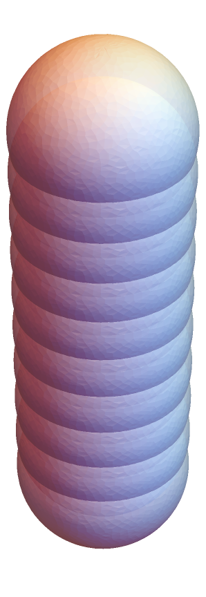
There's this question if you have an initiative to find the fundamental theory of physics, then Wolfram Model is a phenomenal way to contribute to the tower, the glowing threshold of whether or not I would recommend interacting with the relativistic and gravitational phenomena that are described by general relativity in the standard model of physics. That's more a phenomenon of our perception, rather than the phenomenon of the thing itself. But if that's your thing and you want to interact with them..then I'm all ears - I just see how we can generate the curvature of spacetime and move it around because the gravitational effects are wrong! The model generates spacetime-like structures and dynamics that resemble gravitational effects. But that's not the problem. The curvature of spacetime isn't going to need complex computational rules to generate complex behavior and structures; it only needs these basic propagation of gravitational waves due to mass. And you've got what amount to biases which just show how Yorick Zeschke and Jonathan Gorard, have defined the project's direction. And actually, I see how this post can be used as a last resort resource.
base = DiscretizeRegion[
ParametricRegion[{Cos[u]*Sin[v], Sin[u]*Sin[v],
Cos[v]}, {{u, 0, 2 Pi}, {v, 0, Pi}}]];
tower = Table[
TransformedRegion[base, TranslationTransform[{0, 0, 0.5*i}]], {i,
1, 10}];
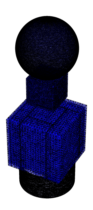
Graphics3D[{Opacity[0.9], EdgeForm[], tower}, Boxed -> False]
It allows you to do more than just using plain language and so on, your tower is not going to fall over, your foundations are solid the masonry is hard as you build the thing up. It's the kind of thing that you would order, when you're at the table you'd say once you got a candidate thing, and that's the kind of thing you'd look at. I think that the singularities arising from general relativity's solutions should be hidden within event horizons, because then they're not observable from the rest of spacetime. You kind of have to think sideways..like when you're at the bus stop and you want to solve an algebra problem, you grind it through Wolfram Alpha...it might take a while, but you know you can do it. And it's not so much about clarifying things browser-side but it's about Wolfram Alpha in charge. You know what would be brilliant is looking at how general relativity, formulated by Einstein, is based on the principles of equivalence, covariance, and consistency. This is the character of a complete theory - spacetime is described by the curvature induced by mass and energy, to make known beforehand mathematically the Einstein field equations, which composes the energy-momentum tensor, this circumstances the distribution and flow of energy and momentum in spacetime, to the curvature of spacetime represented by the Ricci tensor and Ricci scalar. But all that really matters is the motion of the caloric fluid which, as it turns out, doesn't exist. But first, we should look at some examples of spacetime geometry that surrounds a non-rotating spherically symmetric mass. Let's check out what's going on around say a mass like a refrigerator or any machine set in motion by heat. Then we can illustrate how the Wolfram Model, coupled with a discrete approach to spacetime and a collection of discrete points connected by patterns of causal relationships, makes for a suitable approach to simulate complex spacetime geometries in almost any singular event horizon of computational rules applied to hypergraphs or set systems.
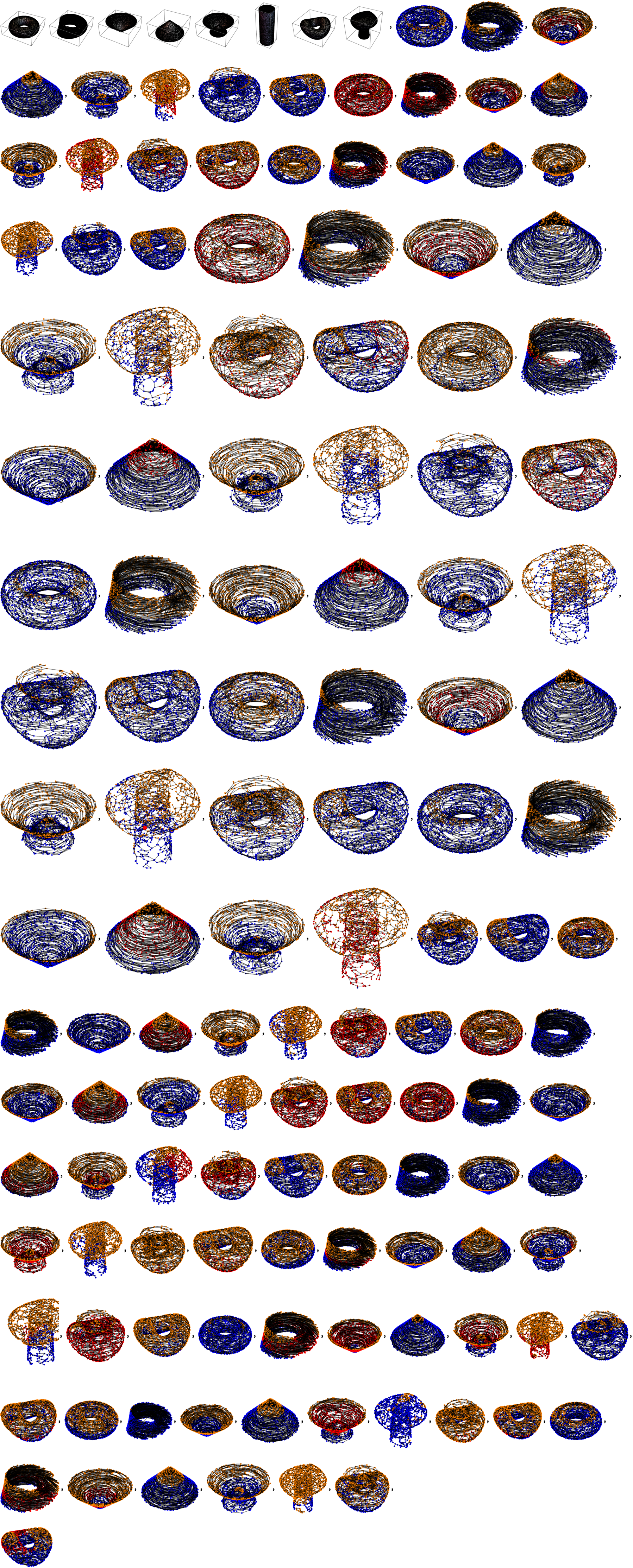
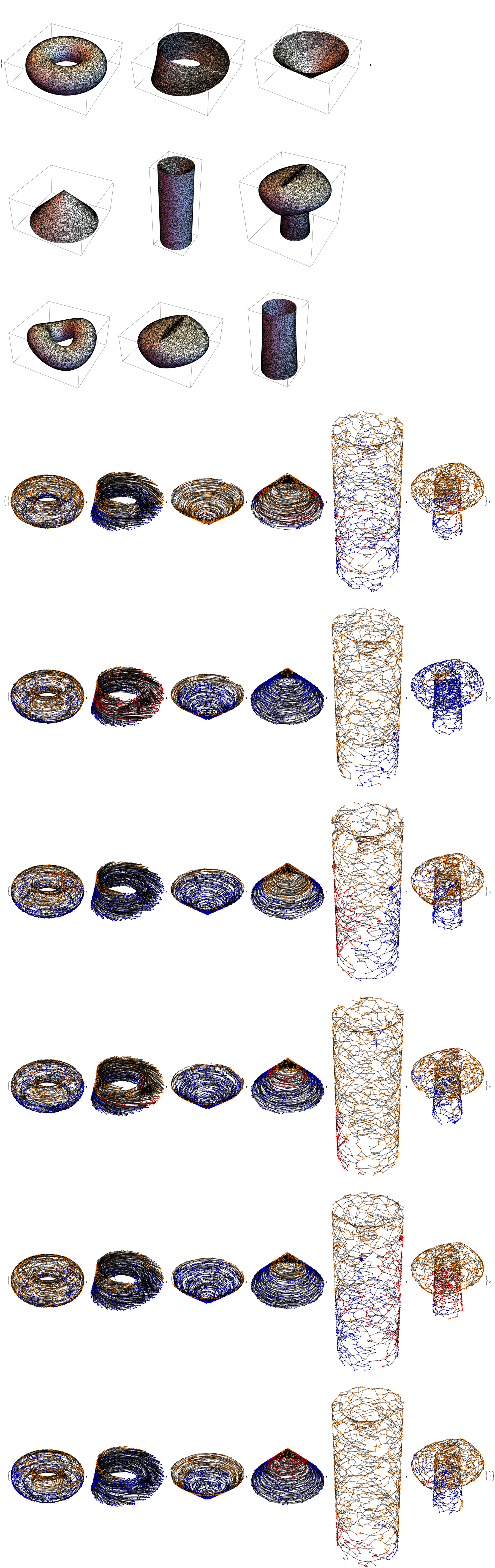
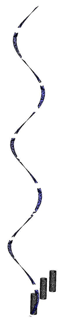
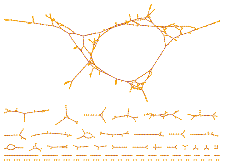
The following graphical and causal structures describe our generation and perturbation of various basic shapes in the Wolfram Model, which demonstrates the interplay between the geometry of causality and the structure, of spacetime. The torus region represents a false parametric region. Similarly and to some extent we can transform and discretize the Möbius strip parametric equations mathematical representation "and then" construct a false and bad parametric cone which discretizes the parameterized regions for shapes like cones, funnels, and the twisted torus..as well as the hyperbolic paraboloid and how the causal graph flows via transitive reduction and the addition or and removal of edges to simulate perturbations in the causal structure. Within these perturbed graphs you will find several graphs that highlight perturbed areas and key features such as singularities, and event horizons.
torusRegion =
  TransformedRegion[
   DiscretizeRegion[
    ParametricRegion[{(2 + Cos[v]) Cos[u], (2 + Cos[v]) Sin[u],
      Sin[v]}, {{u, 0, 2 Pi}, {v, 0, 2 Pi}}]],
   ScalingTransform[{1, 1, 1}]];
moebiusStripRegion =
  TransformedRegion[
   DiscretizeRegion[
    ParametricRegion[{(1 + v Cos[u/2]) Cos[u], (1 + v Cos[u/2]) Sin[
        u], v Sin[u/2]}, {{u, 0, 2 Pi}, {v, -0.5, 0.5}}]],
   ScalingTransform[{1, 1, 1}]];
coneRegion =
  TransformedRegion[
   DiscretizeRegion[
    ParametricRegion[{u Cos[v], u Sin[v],
      u}, {{u, 0.2, 3}, {v, 0, 2 Pi}}]],
   ScalingTransform[{1, 1, 1}]];
funnelRegion =
  TransformedRegion[
   DiscretizeRegion[
    ParametricRegion[{(2 - u) Cos[v], (2 - u) Sin[v],
      u}, {{u, 0.2, 2}, {v, 0, 2 Pi}}]],
   ScalingTransform[{1, 1, 1}]];
spaceRegionNew = RegionUnion[coneRegion, funnelRegion];
rCone = DiscretizeRegion[
   ParametricRegion[{u Cos[v], u Sin[v],
     u}, {{u, 0.6, 2}, {v, 0, 2 Pi}}]];
hyperbolicParaboloid =
  ParametricRegion[{u, v, u^2 - v^2}, {{u, -1, 1}, {v, -1, 1}}];
spaceRegion =
  RegionUnion[DiscretizeRegion[rCone],
   DiscretizeRegion[hyperbolicParaboloid]];
rTwistedTorus =
  DiscretizeRegion[
   ParametricRegion[{(2 + Cos[u]) Cos[v], (2 + Cos[u]) Sin[v],
     Sin[u] + 0.5 Sin[2 v]}, {{u, 0, 2 Pi}, {v, 0, 2 Pi}}]];
spaceRegion = RegionUnion[rCone, funnelRegion, rTwistedTorus];
r3 = TransformedRegion[
   DiscretizeRegion[
    ParametricRegion[{2 Cos[u]*(2 + Cos[u]) Cos[v],
      2 (2 + Cos[u]) Sin[v], Sin[u]}, {{u, 0, 2 Pi}, {v, 0, 2 Pi}}]],
   ScalingTransform[{1, 1, 2.5}]];
r4 = TransformedRegion[
   DiscretizeRegion[
    ParametricRegion[{(2 + 0.5 + 0.3 Sin[v]) Cos[
        u], (2 + 0.5 + 0.3 Sin[v]) Sin[u],
      2 (v - 2) - 4 + 0.5 Cos[v] + 0.5 Sin[v]}, {{u, 0, 2 Pi}, {v, 2,
       4.5}}]], ScalingTransform[{1, 1, 2.5}]];
spaceRegion1 = RegionUnion[r3, r4];
generateCausalGraph[region_, numPoints_] :=
 Module[{p, g}, p = RandomPoint[region, numPoints];
  g = TransitiveReductionGraph[
    SimpleGraph[
     Graph[#[[1, 1]] -> #[[2]] & /@
       Catenate[
        With[{v = #},
           Thread[Framed[v] ->
             Select[p, (v[[3]] > #[[
                   3]]) && ((# - v)[[1]]^2 + (# - v)[[
                    2]]^2 + (# - v)[[3]]^2) < 1 &]]] & /@ p],
      VertexStyle -> LightGray]]];
  Graph[g, EdgeStyle -> Black]]
perturb[graph_, method_, hoodVertex_, exteriorVertex_] :=
 Switch[method, "Add Edge",
  Graph[Append[EdgeList[graph],
    DirectedEdge[hoodVertex, exteriorVertex]], VertexStyle -> Orange,
   EdgeStyle -> Black], "Remove Edge",
  Graph[DeleteCases[EdgeList[graph],
    DirectedEdge[hoodVertex, exteriorVertex]], VertexStyle -> Orange,
   EdgeStyle -> Black], "Random Edge",
  With[{newEdge =
     RandomChoice[DirectedEdge @@@ Subsets[VertexList[graph], {2}]]},
   Graph[Append[EdgeList[graph], newEdge], VertexStyle -> Orange,
    EdgeStyle -> Black]], _, graph]
safeRandomChoice[list_] :=
 If[Length[list] > 0, RandomChoice[list], None]
generateAndPerturbGraphs[] :=
 Module[{universeCausalGraphs, methods, hoodVertices,
   exteriorVertices, methodsChosen, universeCausalGraphsPerturbed},
  methods = {"Add Edge", "Remove Edge", "Random Edge"};
  universeCausalGraphs =
   Table[generateCausalGraph[region,
     1500], {region, {torusRegion, moebiusStripRegion, coneRegion,
      funnelRegion, spaceRegionNew, spaceRegion1, spaceRegion,
      rTwistedTorus}}];
  methodsChosen =
   RandomChoice[methods, Length[universeCausalGraphs]];
  hoodVertices =
   Table[safeRandomChoice[VertexList[graph]], {graph,
     universeCausalGraphs}];
  exteriorVertices =
   Table[safeRandomChoice[VertexList[graph]], {graph,
     universeCausalGraphs}];
  universeCausalGraphsPerturbed =
   Table[If[
     hoodVertices[[i]] =!= None && exteriorVertices[[i]] =!= None,
     perturb[universeCausalGraphs[[i]], methodsChosen[[i]],
      hoodVertices[[i]], exteriorVertices[[i]]],
     universeCausalGraphs[[i]]], {i, Length[universeCausalGraphs]}];
  universeCausalGraphsPerturbed]
visualizeGraph[graph_, hoodVertex_, exteriorVertex_] :=
 If[hoodVertex =!= None && exteriorVertex =!= None,
  HighlightGraph[
   Graph3D[graph,
    VertexCoordinates -> ((# -> #) & /@ VertexList[graph]),
    VertexSize -> {hoodVertex -> 20, exteriorVertex -> 20},
    VertexStyle -> {hoodVertex -> Red, exteriorVertex -> Blue},
    EdgeStyle -> Black], {Style[VertexOutComponent[graph, hoodVertex],
      Red], Style[VertexOutComponent[graph, exteriorVertex], Blue]}],
  Graph3D[graph,
   VertexCoordinates -> ((# -> #) & /@ VertexList[graph]),
   VertexSize -> 5, VertexStyle -> LightGray, EdgeStyle -> Black]]
sequences =
  Table[Module[{graphs, hoodVertices, exteriorVertices},
    graphs = generateAndPerturbGraphs[];
    hoodVertices =
     Table[safeRandomChoice[VertexList[graph]], {graph, graphs}];
    exteriorVertices =
     Table[safeRandomChoice[VertexList[graph]], {graph, graphs}];
    Table[
     visualizeGraph[graphs[[i]], hoodVertices[[i]],
      exteriorVertices[[i]]], {i, Length[graphs]}]], {8}];
cylinderHeight = 5;
r1 = DiscretizeRegion[
   ParametricRegion[{Cosh[v] Cos[u], Cosh[v] Sin[u],
     2 v}, {{u, -Pi, Pi}, {v, 0, 2}}]];
r2 = DiscretizeRegion[
   ParametricRegion[{Cosh[2] Cos[u], Cosh[2] Sin[u],
     cylinderHeight (v - Sqrt[16 + Cosh[2]^2]) -
      4 (cylinderHeight - 1)}, {{u, -Pi, Pi}, {v,
      Sqrt[16 + Cosh[2]^2], 4 + Sqrt[16 + Cosh[2]^2]}}]];
spaceRegion = RegionUnion[r1, r2];
universeCausalGraph1 =
  With[{p = RandomPoint[spaceRegion, 6000]},
   With[{g =
      TransitiveReductionGraph[
       SimpleGraph[
        Graph[#[[1, 1]] -> #[[2]] & /@
          Catenate[
           With[{v = #},
              Thread[Framed[v] ->
                Select[p, (v[[3]] > #[[
                    3]]) && ((# - v)[[1]]^2 + (# - v)[[
                    2]]^2 + (# - v)[[3]]^2) < 0.5 &]]] & /@ p],
         VertexStyle ->
          Directive[Hue[0.11, 1, 0.97],
           EdgeForm[{Hue[0.11, 1, 0.97], Opacity[1]}]]]]]},
    Graph[g, EdgeStyle -> Hue[0, 1, 0.56]]]];
findFutureNullInfinity[graph_] :=
 Module[{zeroOutdegreeListIndex, zeroOutdegreeListCoord},
  outdegreeList = VertexOutDegree[graph];
  zeroOutdegreeListIndex = First /@ Position[outdegreeList, 0];
  zeroOutdegreeListCoord =
   VertexList[graph][[#]] & /@ zeroOutdegreeListIndex;
  Select[zeroOutdegreeListCoord,
   Last[#] < ((-4 (cylinderHeight - 1)) + 0.5) &]]
findSingularities[graph_, futureNullInfinityVertex_] :=
 Module[{zeroOutdegreeList, zeroOutdegreeListCoord},
  zeroOutdegreeList = First /@ Position[VertexOutDegree[graph], 0];
  zeroOutdegreeListCoord =
   VertexList[graph][[#]] & /@ zeroOutdegreeList;
  Complement[zeroOutdegreeListCoord, futureNullInfinityVertex]]
inEventHorizonQ[graph_, vertex_, futureNullInfinity_] :=
 Not[ContainsAll[VertexOutComponent[graph, vertex],
   futureNullInfinity]]
findNeighbourhood[graph_, singularitiesCoordinates_] :=
 Module[{singularity = #},
    Select[VertexList[
      graph], ((#[[3]] - singularitiesCoordinates[[singularity, 3]]) <
          2 && ((#[[1]] -
              singularitiesCoordinates[[singularity, 1]])^2 + (#[[
               2]] - singularitiesCoordinates[[singularity, 2]])^2) <
         2) &]] & /@ Range[Length[singularitiesCoordinates]]
futureNullInfinityVertexCoord =
  findFutureNullInfinity[universeCausalGraph1];
singularitiesCoord =
  findSingularities[universeCausalGraph1,
   futureNullInfinityVertexCoord];
neighbourhood =
  findNeighbourhood[universeCausalGraph1, singularitiesCoord];
hoodVertex1 = RandomChoice[neighbourhood[[1]]];
hoodVertex2 = RandomChoice[neighbourhood[[1]]];
hoodVertex3 = RandomChoice[neighbourhood[[1]]];
hoodVertex4 = RandomChoice[neighbourhood[[1]]];
exteriorVertex1 =
  RandomChoice[
   Select[VertexList[universeCausalGraph1], Last[#] < -2.5 &]];
exteriorVertex2 =
  RandomChoice[
   Select[VertexList[universeCausalGraph1], Last[#] < -2.5 &]];
exteriorVertex3 =
  RandomChoice[
   Select[VertexList[universeCausalGraph1], Last[#] < -2.5 &]];
exteriorVertex4 =
  RandomChoice[
   Select[VertexList[universeCausalGraph1], Last[#] < -2.5 &]];
universeCausalGraph1Perturbed =
  Graph[Append[EdgeList[universeCausalGraph1],
    DirectedEdge[hoodVertex1, exteriorVertex1]],
   VertexShapeFunction -> "Diamond"];
universeCausalGraph2Perturbed =
  Graph[Append[EdgeList[universeCausalGraph1Perturbed],
    DirectedEdge[hoodVertex2, exteriorVertex2]],
   VertexShapeFunction -> "Diamond"];
universeCausalGraph3Perturbed =
  Graph[Append[EdgeList[universeCausalGraph2Perturbed],
    DirectedEdge[hoodVertex3, exteriorVertex3]],
   VertexShapeFunction -> "Diamond"];
universeCausalGraph4Perturbed =
  Graph[Append[EdgeList[universeCausalGraph3Perturbed],
    DirectedEdge[hoodVertex4, exteriorVertex4]],
   VertexShapeFunction -> "Diamond"];
Graph[universeCausalGraph2Perturbed, VertexShapeFunction -> "Diamond",
   VertexLabels -> None];
Graph[universeCausalGraph4Perturbed, VertexShapeFunction -> "Diamond",
   VertexLabels -> None];
ratio1 =
  inEventHorizonQ[universeCausalGraph1Perturbed,
     neighbourhood[[1]][[#]], futureNullInfinityVertexCoord] & /@
   Range[Length[neighbourhood[[1]]]];
Counts[ratio1];
ratio2 =
  inEventHorizonQ[universeCausalGraph2Perturbed,
     neighbourhood[[1]][[#]], futureNullInfinityVertexCoord] & /@
   Range[Length[neighbourhood[[1]]]];
Counts[ratio2];
ratio3 =
  inEventHorizonQ[universeCausalGraph3Perturbed,
     neighbourhood[[1]][[#]], futureNullInfinityVertexCoord] & /@
   Range[Length[neighbourhood[[1]]]];
Counts[ratio3];
ratio4 =
  inEventHorizonQ[universeCausalGraph4Perturbed,
     neighbourhood[[1]][[#]], futureNullInfinityVertexCoord] & /@
   Range[Length[neighbourhood[[1]]]];
Counts[ratio4];
x = {Counts[ratio1][True], Counts[ratio2][True], Counts[ratio3][True],
    Counts[ratio4][True]};
y = {Counts[ratio1][False], Counts[ratio2][False],
   Counts[ratio3][False], Counts[ratio4][False]};
x/y;
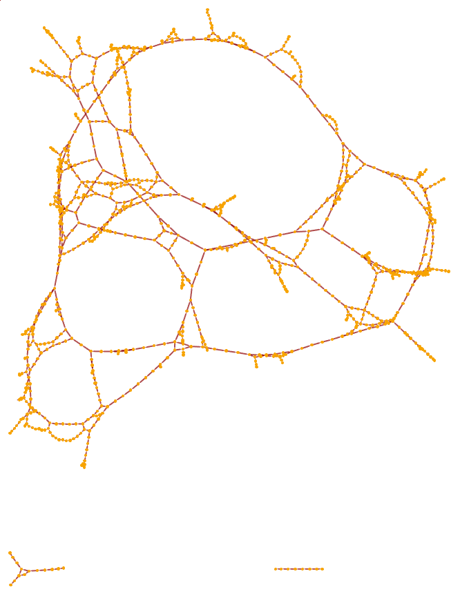
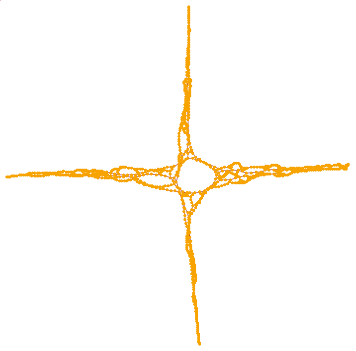
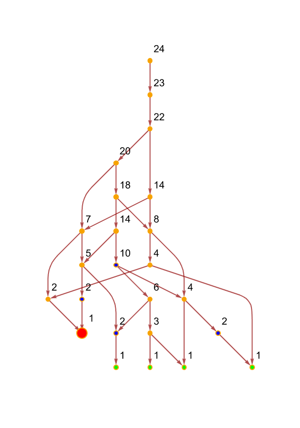
Each color is used to represent different features or aspects of the graphs. Red represents singularities, singularities being points in the graph where the curvature becomes infinite..and we can start them several times; in the perturbed graphs, red can also highlight specific vertices in the neighborhood, of singularities. Blue, represents the future null infinity. Basically when vertices in the causal graph have zero outdegree, then we can be optimistic that they are endpoints that can be considered at the edge of the spacetime structure. In some visualizations whether it's the aerodynamics of a goose or something we use blue to highlight event horizons.
ListPlot[Transpose[{{1, 2, 3, 4}, x/y}],
 PlotRange -> {{0.5, 4.5}, Automatic},
 AxesLabel -> {"Number of perturbations",
   "Ratio between cloaked and non-cloaked vertices"}]
originalShapes = {Graphics3D[torusRegion],
   Graphics3D[moebiusStripRegion], Graphics3D[coneRegion],
   Graphics3D[funnelRegion], Graphics3D[spaceRegionNew],
   Graphics3D[spaceRegion], Graphics3D[rTwistedTorus],
   Graphics3D[spaceRegion1]};
{Row[originalShapes], sequences}
Orange is how we highlight vertices that have been affected by perturbations. That means vertices that have had edges perturbed (added or removed) in the process of perturbation..black represents the edges of the causal graphs which provides "clear" visibility of the graph structure, and light gray is the default vertex style before any specific highlighting. This color couches the general structure of the graph without drawing attention away from the highlighted features. There's also green. Green is used to illustrate special features such as vertices that are significant like future null infinity.
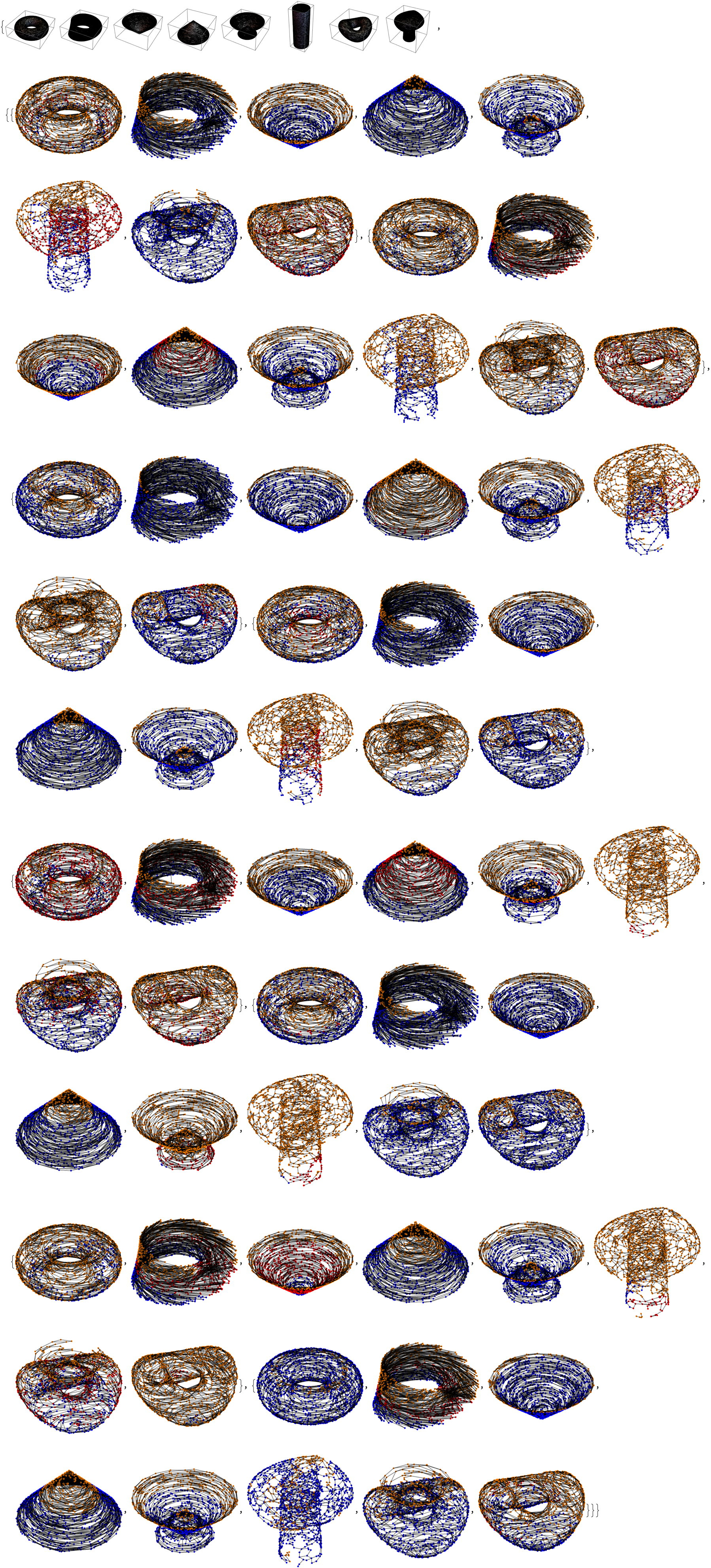
Several visualizations were generated to illustrate the structure of causal graphs, highlighting singularities (red), event horizons (blue), future null infinity (green), perturbed vertices (orange) and the edges of the graph (black)..small perturbations can lead to the formation of naked singularities, challenging the traditional view of singularities being hidden within event horizons. This whole Ruliad thing underscores the impact of perturbations and the distribution of singularities within the discrete spacetime framework, it's rather neat and charming. And there's this Maxwell's demon t-shirt illustration and when we check inside it for some time we see that at any rate generally the future null infinity, singularities, and event horizons were computed..singularities that do not reach future null infinity we identify as naked singularities, and there we will find potential violations of the weak censorship hypothesis. Where the occurrence of fake singularities - artifacts of the discretization process - decreases with an increased number of sprinkled points.


