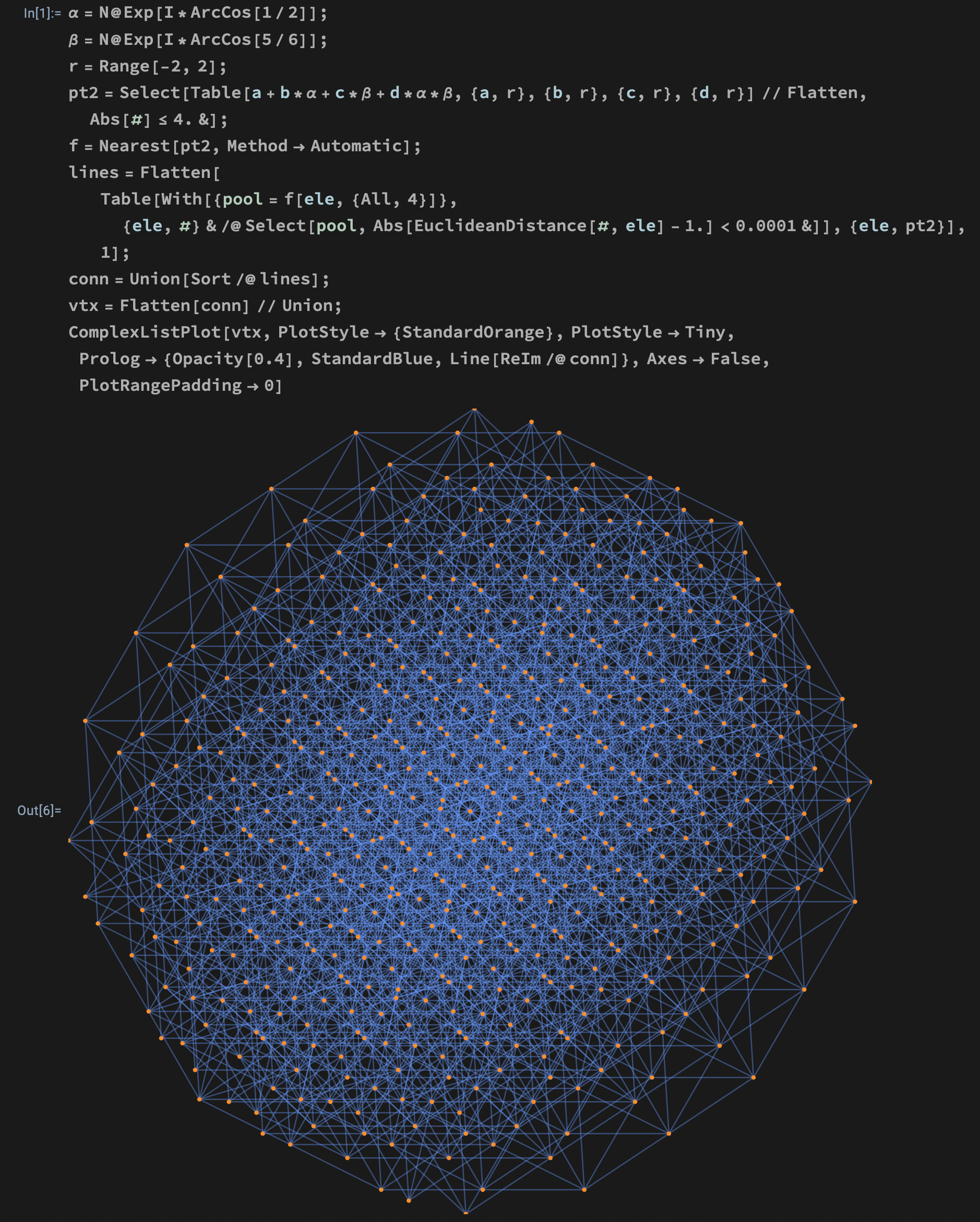
The code here reconstructs the exact same optimal configuration shown on the right-hand side of this Twitter/X post using Moser ring:
\[Alpha]=N@Exp[I*ArcCos[1/2]];
\[Beta]=N@Exp[I*ArcCos[5/6]];r=Range[-2,2];
pt2=Select[Table[a+b*\[Alpha]+c*\[Beta]+d*\[Alpha]*\[Beta],{a,r},{b,r},{c,r},{d,r}]//Flatten,Abs[#]<=4.&];
f=Nearest[pt2,Method->Automatic];
lines=Flatten[
Table[With[{pool=f[ele,{All,4}]},{ele,#}&/@Select[pool,Abs[EuclideanDistance[#,ele]-1.]<0.0001&]],{ele,pt2}],1];
conn=Union[Sort/@lines];
vtx=Flatten[conn]//Union;
ComplexListPlot[vtx,PlotStyle->{StandardOrange},PlotStyle->Tiny,Prolog->{Opacity[0.4],StandardBlue,Line[ReIm/@conn]},Axes->False,PlotRangePadding->0]