High-order series solution of the ODE around x=0 followed by a Pade approximation. difference calculates the difference of the approximation to the right boundary value. It also returns the actual Pade approximation.

difference[\[Alpha]In_Real,\[Xi]_,{prec_, pdO_}] := 
Module[{\[Alpha]=SetPrecision[\[Alpha]In, prec],diff,sol,series,pd,u,x,\[Delta]},  
series=\[Alpha] x -\[Alpha]/8  x^3 ;
Do[diff=u''[x]+u'[x]/x-u[x]/x^2+u[x]-u[x]^3 /.
           u->(Function@@{x,series+C x^M+O[x]^(M+1)});
 series=series  + Together[C x^M /. First[Solve[diff[[3,1]]==0,C]]],{M,5,2pdO+5,2}];
pd=PadeApproximant[series,{x,0,{pdO,pdO}}];
stepData={\[Alpha],\[Delta]=Tanh[10/Sqrt[2]] - pd/. x->10};
{\[Delta], pd /. x -> \[Xi]}
]

Example

difference[0.58318 , x, {20, 20}]

{0.2435578857088556, (0.58318000000000003 x + 0.27407625855333046 x^3 + 0.051256728918896911 x^5 + 0.0048322482238297771 x^7 + 0.00023632082879286407 x^9 + 5.1729410403285544*10^-6 x^11 + 8.2185843137751949*10^-9 x^13 - 1.06931812684189022*10^-9 x^15 - 2.2863733027673254*10^-12 x^17 + 7.6295697669084428*10^-14 x^19)/(1 + 0.59496854925294154 x^2 + 0.142883728435766338 x^4 + 0.0176772849277092897 x^6 + 0.00118228825938525016 x^8 + 0.000039832791262778028 x^10 + 4.5345802881727914*10^-7 x^12 - 5.5226863238549098*10^-9 x^14 - 9.7254616067217217*10^-11 x^16 + 6.0544145050658359*10^-13 x^18 + 3.9887426264821583*10^-15 x^20)}

Find slope at x=0 to any desired precision (by increasing prec and pdO). Say 15 digits.

Monitor[
 fr = FindRoot[
    difference[\[Alpha], x, {100, 200}][[1]], {\[Alpha], 0.5831, 0.5832}, WorkingPrecision -> 60, PrecisionGoal -> 16, 
    Method -> "Brent", Evaluated -> False];,
 stepData]

fr

{\[Alpha] -> 0.583189634418924769412413009673771234659851269345508491782915}

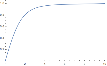
The rational approximate solution.

uSol = difference[\[Alpha] /. fr, x, {100, 200}][[2]];
Plot[Evaluate[uSol], {x, 0, 10}, PlotRange -> All]

Check right boundary condition

(uSol /. x -> 10) - Tanh[10/Sqrt[2]]

-2.6496232607434627305318392508171048229727621206337120044345649125837*10^-27

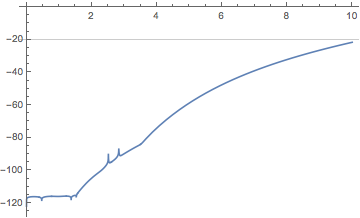
Check ODE. It is fulfilled to 20 digits everywhere.

odeDiff = u''[x] + u'[x]/x - u[x]/x^2 + u[x] - u[x]^3 /. u -> Function[x, Evaluate[uSol]];

Quiet[ Plot[Log10[Abs[odeDiff]], {x, 0, 10}, WorkingPrecision -> 200, 
  GridLines -> {None, {-20}}, PlotRange -> {Full, {All, 0}}], Plot::precw]

Notebook is attached.

Attachments:

Ah, ok! When deriving the new domain, I had a typo and used $t = e^{-x}$ instead of $x = e^{-t}$...

I attacked this problem by making the substitution $x = e^{-t}$. When subbing for the independent variable, we need to make careful use of the chain rule to express $u(x), u'(x), u''(x)$ in terms of $u(t), u'(t), u''(t)$.

ode = u''[x]+(u'[x]/x)-(u[x]/(x^2))+u[x]-u[x]^3 == 0;
sub = Exp[-t];

newode = ode /. {
    u[x] -> u[t],
    u'[x] -> u'[t]/D[sub, t],
    u''[x] -> (u''[t] - D[sub, {t, 2}] u'[t]/D[sub, t])/D[sub, t]^2,
    x -> sub
}

u[t] - E^(2 t) u[t] - u[t]^3 - E^(2 t) u'[t] + E^(2 t) (u'[t] + u''[t]) == 0

sol = NDSolveValue[{newode, u[1] == 0, u[0] == 1}, u[t], t] /. t -> Exp[-x];
sol /. x -> 0

0.

sol /. x -> 10^15

1.

Plot[Evaluate[sol], {x, 0, 10}, PlotRange -> All]

Here's my issue though... If I plug this solution into the original ODE, I don't get zero, so I think I did something wrong but I can't figure out where. In fact I am having the same issue with Hans Dolhaine's solution he posted above (his is sol2 in the plot below).

Maybe someone here can figure out where I went wrong? I feel it's a simple oversight.

Plot[Evaluate[{
   D[sol, {x, 2}] + (D[sol, x]/x) - (sol/x^2) + sol - sol^3,
   D[sol2, {x, 2}] + (D[sol2, x]/x) - (sol2/x^2) + sol2 - sol2^3
 }], {x, 4, 20}, PlotRange -> All]

But can I use NDSolve to solve the equations with u[x=0] = 0 and u[x=1000] = 1 (for example)? How? I'm not an expert in Mathematica. Thanks a lot.

They used the so called "Chebyshev method", but I don't know how it works.

Unfortunately there is a mistake in the last plot-command, working with Exp[ - x^2 ] instead of Exp[ - x^1.3 ] which was used to solve the differential equation. With the last setting the approach doesn't work.

But another question: the differentials in the original equation are obviously the laplacian in cylindical coordinates. The function part is

u[x] - u[x]/x^2 - u[x]^3

and this may be written as

-u[x] (u[x] - Sqrt[-1 + x^2]/x) (u[x] + Sqrt[-1 + x^2]/x)

What does that mean for the allowed values of x? If u is real then x > 1 ?

Well, not monotone for small values of x, but......

eq1 = u''[x] + (u'[x]/x) - (u[x]/(x^2)) + u[x] - u[x]^3;
uu[x_] := 1 - v[x] Exp[-x^1.3];
eq2 = x^2 FullSimplify[eq1 /. u -> uu];
eq2a = FullSimplify[Solve[eq2 == 0, v''[x]][[1, 1]]] /. Rule -> Equal
eps = 10^-3;
sol = v /. 
  NDSolve[{eq2a, v[eps] == 1, v'[eps] == -.1}, v, {x, eps, 50}, 
    Method -> "ExplicitRungeKutta"][[1]]
Plot[1 - Exp[-x^2] sol[x], {x, eps, 10}, PlotRange -> All]

Dear Mattia,

a really interesting problem, and I see the point, but what are BC's? And I am somewhat astonished that a quantum-mechanical function does not vanish for x -> infinity.

But besides that I tried a "brute force" solution:

Your original equation was

eq1 = u''[x] + (u'[x]/x) - (u[x]/(x^2)) + u[x] - u[x]^3;

Now I looked for a function (hopefully) converging towards 1 for x -> Infinity. This should workk if v does not grow faster than exp.

uu[x_] := 1 - v[x] Exp[-x]

(Later I tried Exp[ - x^2 ] as well )

This gave a modified differential equation for v[ x ]

 In[3]:= eq2 = x^2 FullSimplify[eq1 /. u -> uu]

  Out[3]= E^(-3 x) (E^(2 x) (1 + x + x^2) v[x] - 3 E^x x^2 v[x]^2 + 
     x^2 v[x]^3 - E^(2 x) (E^x + (1 - 2 x) x 
  \!\(\*SuperscriptBox["v", "\[Prime]",
  MultilineFunction->None]\)[x] + x^2 
  \!\(\*SuperscriptBox["v", "\[Prime]\[Prime]",
  MultilineFunction->None]\)[x]))

Which I tried to solve numerically

eps = 10^-3;
sol = v /. 
  NDSolve[{eq2 == 0, v[eps] == 1, v'[eps] == 0}, v, {x, eps, 5}, 
    Method -> "ImplicitRungeKutta"][[1]]

But even after about 50 minutes of evaluation no result was given back.

Regards Hans

Dear Hans, unfortunately the behavior of the first derivative is unknown. This is a typical Schroedinger problem, in which only BC's are known. Your solution seems to be correct near 0, but the function is monotone and most reach asymptotically 1 at +inf.

Luca, Nice, you avoid the stiffness issue by using a shooting method! How did you find the initial value of 1.11?

Yes, that sounds good. But what if you integtate to, say, x = 10? At least with my system the solution "explodes".

And it shows a peculiar behaviour around 1.11. Just have a try with 1.105 and 1.108 and so on....

Hello Mattia,

as it is a diff.eq. of second order we need to have information about the first derivative as well. And the division by x leads to problems at x == 0. But we could try to start in the vicinity of 0:

eq = u''[x] + (u'[x]/x) - (u[x]/(x^2)) + u[x] - u[x]^3 == 0;
eps = 10^-4;
sol = u /. 
  NDSolve[{eq, u[eps] == 0, u'[eps] == .2}, u, {x, eps, 5}][[1]]
Plot[sol[x], {x, eps, 3}]

Thanks Kay. The equation gives the vortex solution to the GPE, and it represents a wave function for dilute BECs. The domain has not to be necessarily infinite, but big enough. I also have to generalize the method to another equation with is similar, but has a parameter. How have you find the solution u = x^(Sqrt[5]/2 - 1/2)/(B + x^(Sqrt[5]/2 - 1/2)) and the plot (which is exactly what I expected)? What code should I use? (I'm not an expert with Mathematica). Thanks a lot.

Thanks a lot Kay!

keep in mind, my approximation is very rough and not accurate. I'm sure there is a way to get a better solution

DSolve is unlikely to solve equations with nonlinear terms in it