Here is a case which finds after a rather long path into repetition

Graphics[Line[AnglePath[Partition[N[Flatten[
      SubstitutionSystem[Rule[#[[1]], {#[[2]]}] & /@ Partition[First[RealDigits[N[E, 130]]], 2], 
       First [RealDigits[N[1/EulerGamma, 150]]], 146]]], 2]]]]

Want to look into the evil eye? Try

Graphics[Line[AnglePath[Partition[N[Flatten[
      SubstitutionSystem[Rule[#[[1]], {#[[2]]}] & /@ Partition[First[RealDigits[N[\[Pi], 30]]], 2], 
       First [RealDigits[N[1/E, 10]]], 206]]], 2]]]]

or

Graphics[Line[AnglePath[Partition[N[Flatten[
      SubstitutionSystem[Rule[#[[1]], {#[[2]]}] & /@ Partition[First[RealDigits[N[\[Pi], 30]]], 2], 
       First [RealDigits[N[\[Pi]/E, 10]]], 144]]], 2]]]]

Very cool. Udo's example (how can I l write a link that goes to his example?) reminds me of one of Stephen Wolfram's live experiments at the 2015 summer school which might have used SubstitutionSystem, but might have also been even simpler.

Let SubstitutionSystem produce the patterns

Graphics[Line[AnglePath[N[Flatten[SubstitutionSystem[
              Rule[#[[1]], {#[[2]]}] & /@ Partition[First[RealDigits[N[Pi, 30]]], 2], {1}, 44]]]]]]

Graphics[Line[AnglePath[N[Flatten[SubstitutionSystem[
      Rule[#[[1]], {#[[2]]}] & /@ Partition[First[RealDigits[N[E, 30]]], 2], {1}, 45]]]]]]

the circle number $\pi$ gives a rounder picture than the Euler number $e$. One can do thousands of figures

Gaphics[Line[AnglePath[N[Flatten[SubstitutionSystem[
      Rule[#[[1]], {#[[2]]}] & /@ Partition[First[RealDigits[N[Pi, 30]]], 2], {7, 3, 2}, 104]]]]]]

one more

Graphics[Line[AnglePath[N[Flatten[SubstitutionSystem[
      Rule[#[[1]], {#[[2]]}] & /@ Partition[First[RealDigits[N[E, 30]]], 2], First[RealDigits[N[E, 3]]], 45]]]]]]    

imposing as

Or doing something ill-looking

Graphics[Line[AnglePath[N[Flatten[SubstitutionSystem[
      Rule[#[[1]], {#[[2]]}] & /@ Partition[First[RealDigits[N[E, 30]]], 2], First[RealDigits[N[E \[Pi], 133]]], 45]]]]]]

Following cool ideas from Marco's answer I am adding Collatz to my gallery. The longest progression for any initial starting number less than 10 billion it is 9,780,657,631, with 1132 steps. I plot its neighbor 9,780,657,630 too and for 1200 to see the cycle.

data0 = NestList[If[EvenQ[#], #/2, 3 # + 1] &, 9780657630, 1200];
data1 = NestList[If[EvenQ[#], #/2, 3 # + 1] &, 9780657631, 1200];
Graphics[{
  Red, BSplineCurve[Reverse /@ AnglePath[Log@N@data0]],
  Blue, BSplineCurve[Reverse /@ AnglePath[Log@N@data1]]}, 
 ImageSize -> 900, Background -> GrayLevel[.1]]

Do not dwell too long on Collatz though... "Mathematics may not be ready for such problems." ~ Paul Erd?s about the Collatz conjecture

Dear Ed and Vitaliy,

these are beautiful and nicely symmetric curves. I have tried some other, less regular systems. Let's run a chaotic logistic map:

logistmap=NestList[4.*#*(1 - #) &, RandomReal[], 100];

We can plot this:

ListLinePlot[ NestList[4.*#*(1 - #) &, RandomReal[], 100], Mesh -> Full, MeshStyle -> Red]

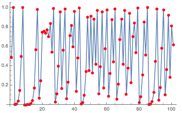
Note that it is a time discrete map in a chaotic regime; the blue line is just to guide the eye. I chose to start at a random initial condition, which is generated by the RandomReal[]. The AnglePath looks like this:

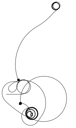
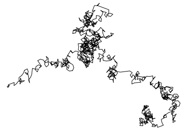
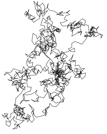
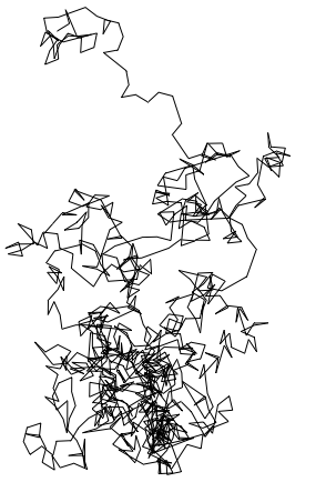
Graphics[Line[AnglePath[NestList[4.#(1 - #) &, RandomReal[], 10000]]]]

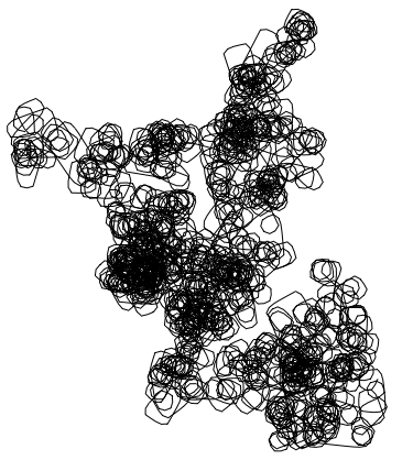
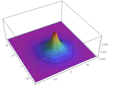
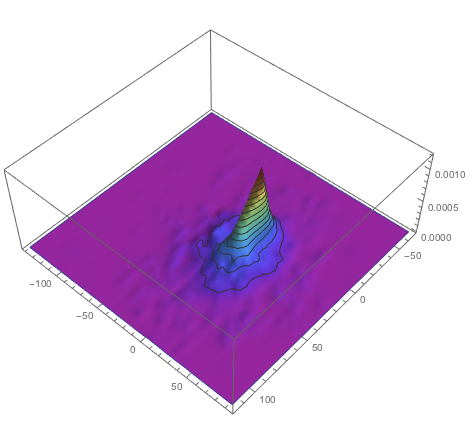
Now, every time you run this, we use a different initial condition, i.e. the path is always different. We could try to figure out where we are on average over, say, 1000 runs and then plot that:

coords = Table[AnglePath[NestList[4.*#*(1 - #) &, RandomReal[], 1000]], {k, 1, 1000}];
SmoothHistogram3D[Flatten[coords, 1], ColorFunction -> "Rainbow"]

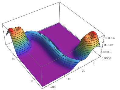
Ok. Let's compare that to Ed's example. All trajectories are the same; it makes no difference but to be consistent with the logistic map example I'll run it 1000 times:

coords2 = Table[AnglePath[N[(7 Sqrt[7] Khinchin Pi E EulerGamma) Range[-2000, 2000]]], {k, 1, 1000}];
SmoothHistogram3D[Flatten[coords2, 1], ColorFunction -> "Rainbow"]

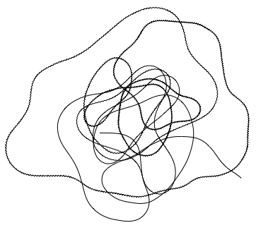
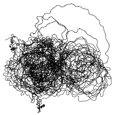
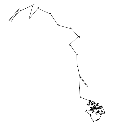
We can now also look at a Levy-flight-like situation:

Graphics[Line[AnglePath[Accumulate@(RandomChoice[{-1, 1}, 1000]*RandomVariate[LevyDistribution[0, 0.0001], 1000])]]]

and

coords3 = Table[AnglePath[Accumulate@(RandomChoice[{-1, 1}, 1000]*RandomVariate[LevyDistribution[0, 0.0001], 1000])], {k, 1,1000}];
SmoothHistogram3D[Flatten[coords3, 1], ColorFunction -> "Rainbow"]

It is very nice that the geometry can represent the dynamics. Of course, it is easy to find something for those who like "patterns and numbers".

Let's look at the digit path of $Pi$.

Graphics[Line[AnglePath[RealDigits[N[Pi, 1000]][[1]]]]]

Then $\sqrt{2}$

Graphics[Line[AnglePath[RealDigits[N[Sqrt[2], 1000]][[1]]]]]

I guess that $e$ is also important:

Graphics[Line[AnglePath[RealDigits[N[Exp[1], 1000]][[1]]]]]

These paths all look quite "random" which is typical for "normal numbers", i.e. numbers the digits of which could come from a random draw of digits. You get beautiful patterns for non-normal numbers like 1/3.

Graphics[Line[AnglePath[RealDigits[N[1/3, 1000]][[1]]]]]

Here's 1/7:

Graphics[Line[AnglePath[RealDigits[N[1/7, 1000]][[1]]]]]

Heres it comes for the inverses of the first 5 primes:

GraphicsRow[Graphics[Line[AnglePath[RealDigits[N[1/#, 1000]][[1]]]]] & /@ Prime[Range[5]]]

Finally, we can look at the patterns in different bases, here for 1/7:

Graphics[Line[AnglePath[RealDigits[N[1/7, 200], #, 200][[1]]]]] & /@ Range[2, 10]

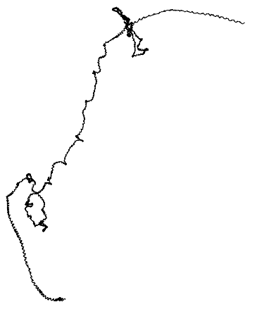
It can also be useful to visualise sound. Here is what a viola looks like:

sndviola = ExampleData[{"Sound", "Viola"}];
Graphics[Line[AnglePath[sndviola[[1, 1, 1]]]]]

An organ is a completely different kettle of fish (I admit that this was not a very common sentence!):

sndorgan = ExampleData[{"Sound", "OrganChord"}];
Graphics[Line[AnglePath[sndorgan[[1, 1, 1]]]]]

This is "Houston we have a problem!":

sndapollo = ExampleData[{"Sound", "Apollo13Problem"}];
Graphics[Line[AnglePath[snd[[1, 1, 1]]]]]

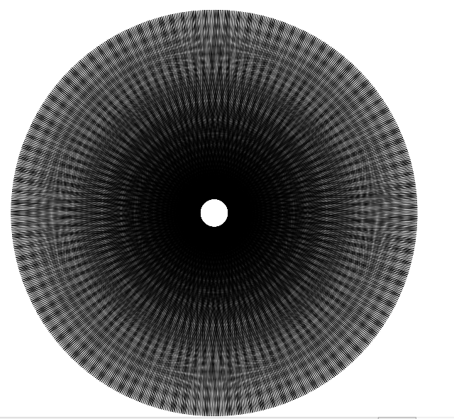
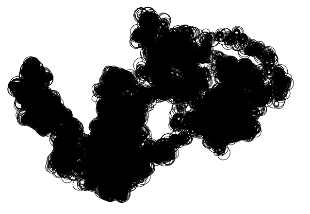
Obviously, this works with images, too. Here is Lena:

Graphics[Line[AnglePath[Flatten[ImageData[ExampleData[{"TestImage", "Lena"}]]]]]]

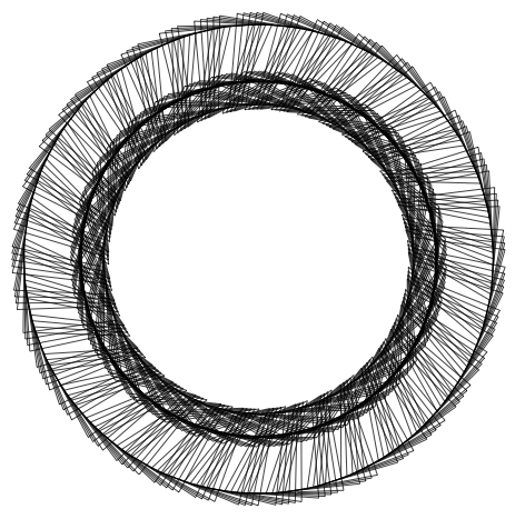
As expected, more regular data

ExampleData[{"TestImage", "ResolutionChart"}]

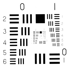
look more regular:

Graphics[Line[AnglePath[Flatten[ImageData[ExampleData[{"TestImage", "ResolutionChart"}]]]]]]

I know that there are many people here who like CellularAutomata. AnglePath can also produce a nice visualisation of the resulting patterns:

Graphics[Line[AnglePath[Flatten[CellularAutomaton[30, {{1}, 0}, 50]]]]]

and

Graphics[Line[AnglePath[Flatten[CellularAutomaton[{1599, {3, 1}}, {Table[1, {1}], 0}, 80]]]]]

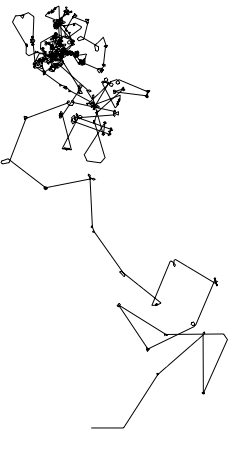
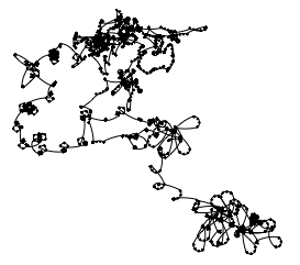
It appears to me that it can even be used for the analysis of graphs.

Graphics[Line[AnglePath[Flatten[Normal[AdjacencyMatrix[RandomGraph[BarabasiAlbertGraphDistribution[100, 2]]]]]]]]

The degree distribution, for example, changes the AnglePaths substantially.

Well, that's all I got for now...

Cheers,

Marco