Group Abstract Group Abstract

Message Boards Message Boards

Determine the equilibrium points of a predator-prey model?

Posted 9 years ago

Hi I am trying to determine the equilibrium points in terms of the nondimensional parameters. the following is the non dimensionalised system:

f[u_, v_] := u (1 - u + (-1 + E^(-u \[Alpha])) v)
g[u_, v_] := v (\[Beta] - E^(-u \[Alpha]) \[Beta] - \[Gamma])

I used the following codes to determine the equilibrium points :

equilibrio = Solve[{f[u, v] == 0, g[u, v] == 0}, {u, v}]

And i get the following error:

'' This system cannot be solved with the methods available to Solve. ''

how can i get the equilibrium points? Please leave your thoughts Thanks Jo

6 Replies

Dear Murray,

you are quite right. My code was incomplete in the sense that it needed the lines from the original post, too. "sols" holds the solutions of the ODEs so that if you execute:

f[u, v] := u (1 - u + (-1 + E^(-u \[Alpha])) v);
g[u, v] := v (\[Beta] - E^(-u \[Alpha]) \[Beta] - \[CapitalGamma]);
sols = NSolve[{f[u, v] == 0, g[u, v] == 0}, {u, v}, Reals];

before the lines I posted, it should work. I noticed that in the original post the result of NSolve was saved in a variable equilibrio, which I renamed to sols. I certainly should have said that.

Sorry, Marco

PS: Note that the definition of the functions is taken from the original. I have not modified the definition of the function so something like:

f[u_, v_] := u (1 - u + (-1 + E^(-u \[Alpha])) v);
g[u_, v_] := v (\[Beta] - E^(-u \[Alpha]) \[Beta] - \[CapitalGamma]);
sols = NSolve[{f[u, v] == 0, g[u, v] == 0}, {u, v}, Reals];

which would look more like a standard definition.

POSTED BY: Marco Thiel

I'm getting errors when I try to evaluate both your Manipulate expressions. For he first:

Part::take: Cannot take positions 1 through 3 in sols. >>
ReplaceAll::reps: {sols[[1;;3]]} is neither a list of replacement rules nor a valid dispatch table, and so cannot be used for replacing. >>

etc.

For the second:

Select::normal: Nonatomic expression expected at position 1 in Select[sols,!MemberQ[#1[[All,2]],Undefined]&]. >>
ReplaceAll::reps: {sols} is neither a list of replacement rules nor a valid dispatch table, and so cannot be used for replacing. >>
ReplaceAll::reps: {!MemberQ[#1[[All,2]],Undefined]&} is neither a list of replacement rules nor a valid dispatch table, and so cannot be used for replacing. >>

etc.

POSTED BY: Murray Eisenberg

Thanks a lot. I am trying to do now the streamplot the method different to you have done and I will comapre with your streamplot. thanks again Jopaul

You might also like this:

Manipulate[
 VectorPlot[{u (1 - u + (-1 + E^(-u \[Alpha]1)) v),  v (\[Beta]1 - E^(-u \[Alpha]1) \[Beta]1 - \[CapitalGamma]1)}, {v, -5, 
   5}, {u, -5, 5}, StreamPoints -> 40, Epilog -> {Red, PointSize[0.02], Point[Evaluate[
      Select[{v, u} /. (sols[[1 ;; 3]] /. {\[Alpha] -> \[Alpha]1, \[Beta] ->  \[Beta]1, \[CapitalGamma] -> \[CapitalGamma]1}), !MemberQ[#, Undefined] &]]]}], {{\[Alpha]1, 0.795}, 0, 2}, {{\[Beta]1, 1.79}, 0, 2}, {{\[CapitalGamma]1, 1.315}, 0, 3}]

enter image description here

Cheers,

M.

PS: This modified version also plots the null-clines and indicates the stability of the fixed points.

Manipulate[
 colors = (Which[(Re[#[[1]]] == 0 && Re[#[[2]]] == 0), Blue, (Re[#[[1]]] < 0 && Re[#[[2]]] < 0), 
              Green, (Re[#[[1]]] > 0 && Re[#[[2]]] > 0), Red, True, Orange] & @
                Eigenvalues[D[{u (1 - u + (-1 + E^(-u \[Alpha])) v), v (\[Beta] - E^(-u \[Alpha]) \[Beta] - \[CapitalGamma])}, {{v, u}}] /. # /. {\[Alpha] -> \[Alpha]1, \[Beta] ->  \[Beta]1, \[CapitalGamma] -> \[CapitalGamma]1}]) & /@ (Select[ (sols \
/. {\[Alpha] -> \[Alpha]1, \[Beta] ->  \[Beta]1, \[CapitalGamma] -> \[CapitalGamma]1}), ! MemberQ[#[[All, 2]], Undefined] &]); 
Show[VectorPlot[{u (1 - u + (-1 + E^(-u \[Alpha]1)) v), v (\[Beta]1 - E^(-u \[Alpha]1) \[Beta]1 - \[CapitalGamma]1)}, {v, -5, 5}, {u, -5, 5}, StreamPoints -> 40, 
   Epilog -> Flatten@{PointSize[0.02], Red, {#[[1]], Point[#[[2]]]} & /@ Transpose[{colors, (Select[{v, u} /. (sols /. {\[Alpha] -> \[Alpha]1, \[Beta] ->  \[Beta]1, \[CapitalGamma] -> \[CapitalGamma]1}), !MemberQ[#, Undefined] &])}]}], ContourPlot[{u (1 - u + (-1 + E^(-u \[Alpha]1)) v) == 0, 
    v (\[Beta]1 - E^(-u \[Alpha]1) \[Beta]1 - \[CapitalGamma]1) == 0}, {v, -5, 5}, {u, -5, 5}, PlotPoints -> 30]], {{\[Alpha]1, 0.795}, 0, 2}, {{\[Beta]1, 1.79}, 0, 
  2}, {{\[CapitalGamma]1, 1.315}, 0, 3}]

enter image description here

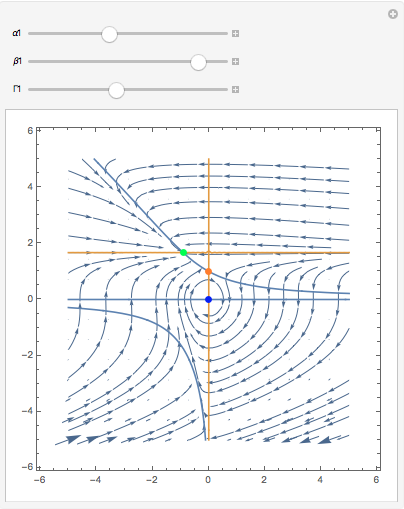
It is not very elegant in terms of the programming, but does the trick. Blue indicates non-hyperbolicity - so we cannot determine the stability using linearisation. Green is stable, orange is a saddle, and red would be unstable in both eigen-directions. Null-clines for the x-direction are in blue and for the y-direction in yellow/gold. Fixed points are where null-clines "of different colour" meet. You will see that in the code I calculate the Jacobian Matrix and evaluate at the fixed points. That means that the program calculates the eigenvalues, that - using the Hartman-Grobman theorem- determine the stability of hyperbolic fixed points.

I hope I haven't made a typo somewhere in the code...

POSTED BY: Marco Thiel

You do know that the definition of a function uses the form f[u,v]:= . . . Write g[u,v]:= . . . on a separate line. Also parentheses are not matching.

POSTED BY: S M Blinder

Hi,

it appears that NSolve does a good job:

f[u, v] := u (1 - u + (-1 + E^(-u \[Alpha])) v);
g[u, v] := v (\[Beta] - E^(-u \[Alpha]) \[Beta] - \[CapitalGamma]);
NSolve[{f[u, v] == 0, g[u, v] == 0}, {u, v}, Reals]

gives

enter image description here

Cheers,

M.

POSTED BY: Marco Thiel
Reply to this discussion
Community posts can be styled and formatted using the Markdown syntax.
Reply Preview
Attachments
Remove
or Discard