Message Boards Message Boards

Improving marksmanship with smooth kernel distribution

Posted 8 years ago

enter image description here

One of the hobbies that I really enjoy is target practice. It requires focus and lots of practice. But most importantly, you need track your improvement (or lack of) objectively.

What better than using the Wolfram Language capabilities to do so!

The following image is a sample of a target placed about 10 yards away.

enter image description here

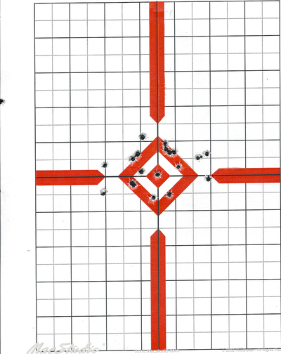
The first two objectives are:

  • Obtain the coordinates of the center of the target
  • Obtain a list of the positions of each impact for further calculations.

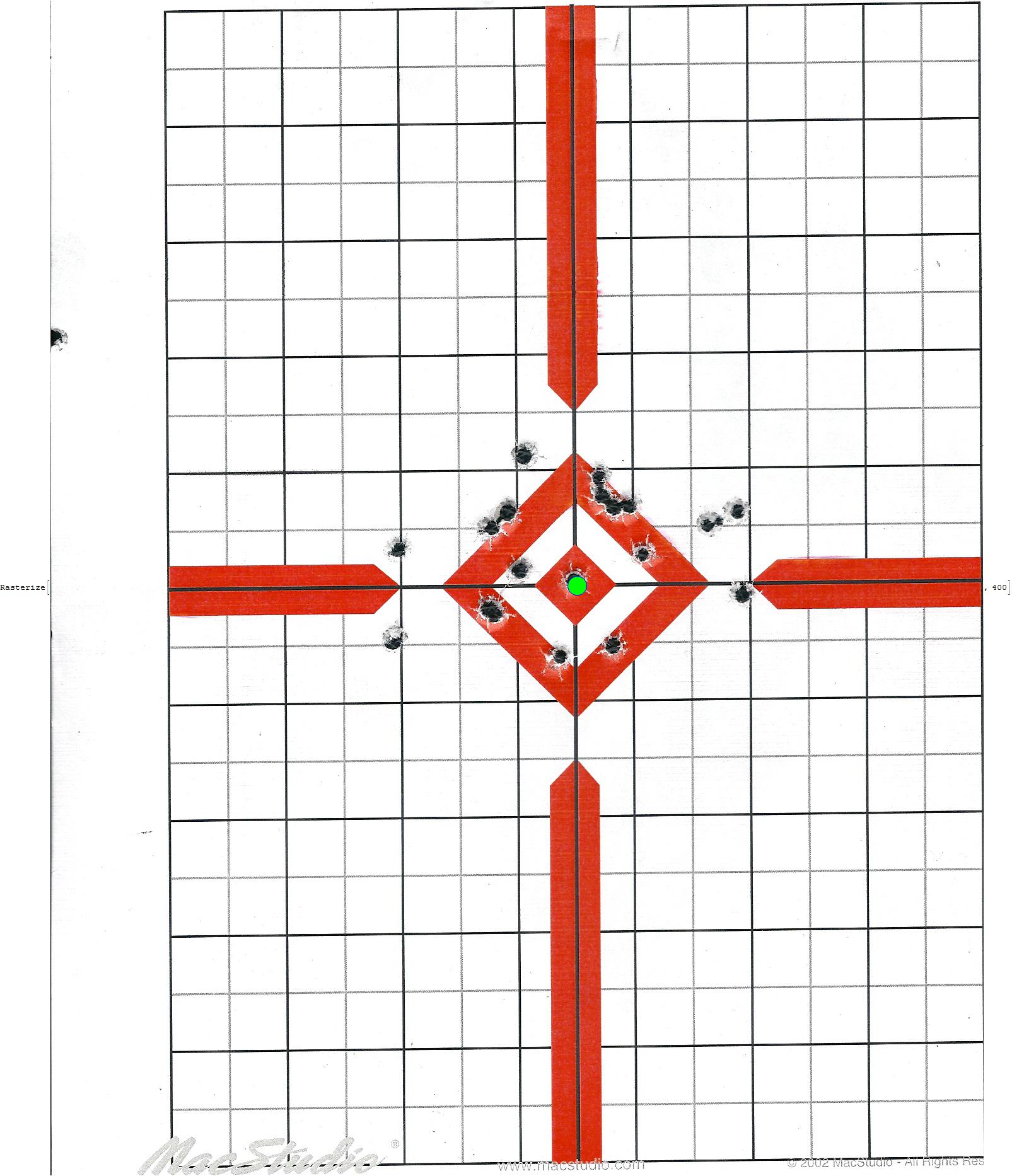
Finding the target center

Let's use an image of the bullseye to locate the center of the target. Using ImageCorrelate will help us do so.

findCenter[img_, kern_] :=  Module[{data}, 
 data = ImageData[
    ImageCorrelate[img, kern, NormalizedSquaredEuclideanDistance], 
    "Byte"]; 
  Rest@Reverse@First@Position[Reverse@data, Min[Flatten[data]]]]

kern = Import["C:\\Users\\Diego\\Documents\\Documents\\Shooting\\10 \yds\\kernel.jpg"];
target = Import["C:\\Users\\Diego\\Documents\\Documents\\Shooting\\10 \yds\\scan0008.jpg"];
findCenter[target, kern]
(*{761, 799}*)
Show[target, Graphics[{Green, Disk[findCenter[target, kern], 10]}]]

enter image description here

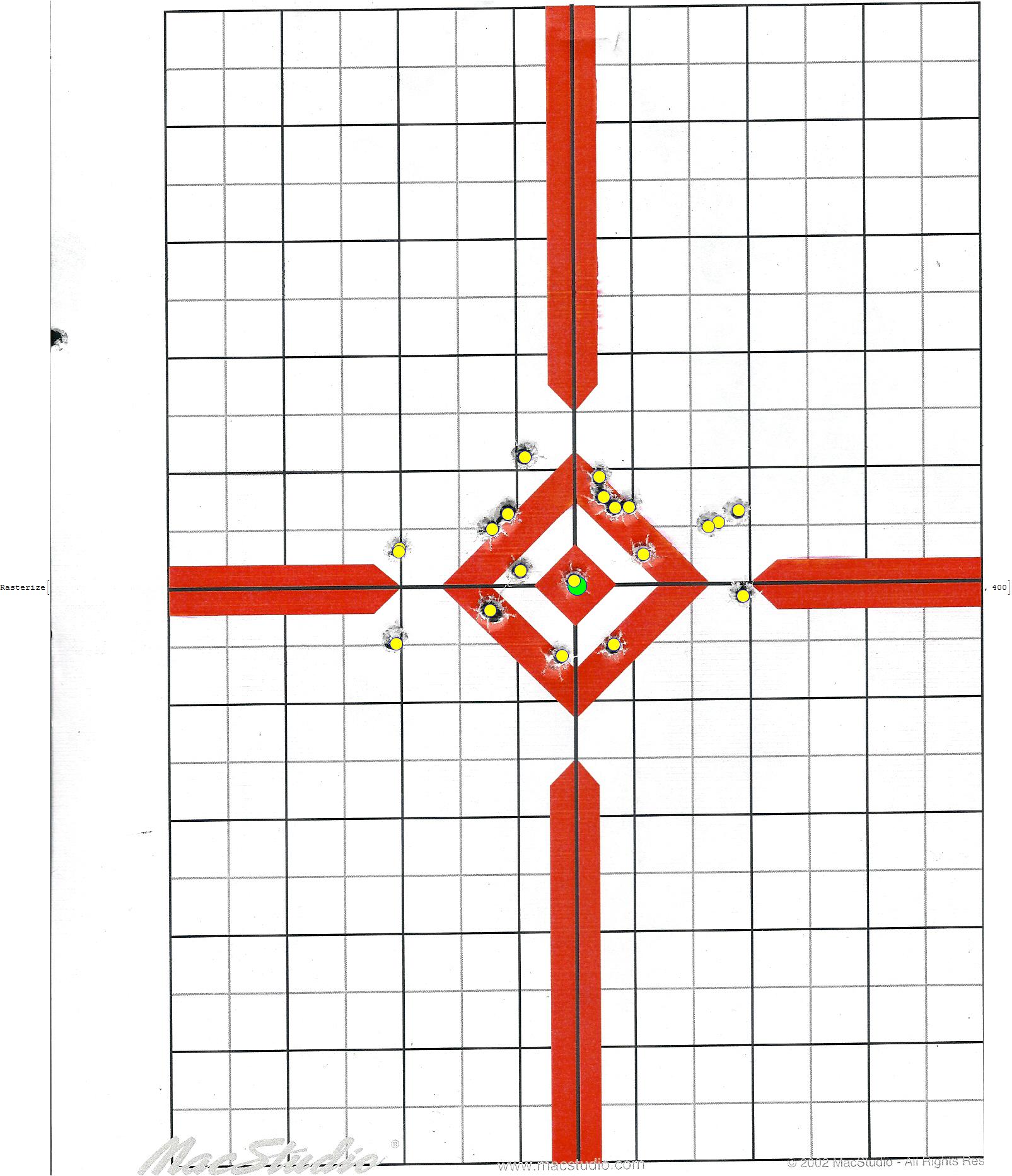
Obtaining the distance of each impact to the center of the target

Using the morphological image processing capabilities of WL we can proceed to extract the positions of each shot. Based on the scanner resolution used to capture the image, the values returned are in cm.

shots[img_, kern_] := 
 Module[{src, red, shotValues, center, values, data},
  red = ColorSeparate[img, "RGB"][[1]]; 
  shotValues = DeleteCases[DeleteCases[
     Last /@ ComponentMeasurements[
       MaxDetect@DistanceTransform@ColorNegate@DeleteSmallComponents@
           Binarize[
            Closing[ImageAdjust[Blur@Blur@Blur@red, {1, 1}], 2]], 
       "Centroid"], {0.5, ___}], {___, 0.5}];
  data = ImageData[ImageCorrelate[img, kern, NormalizedSquaredEuclideanDistance],"Byte"]; 
  center = Rest@
    Reverse@First@Position[Reverse@data, Min[Flatten[data]]];
  values = (# - center)/100 & /@ shotValues]

enter image description here


Exploratory Data Analysis of a practice session

Now that we the functions needed we can process all targets of a given set.

files = FileNames["C:\\Users\\Diego\\Documents\\Documents\\Shooting\\10 \yds\\scan*.jpg"];
imgs = Import[#] & /@ files;
results = Flatten[shots[#, kern] & /@ imgs, 1];
kde = SmoothKernelDistribution[results];
Show[ContourPlot[PDF[kde, {x, y}], {x, -5, 5}, {y, -5, 5}], 
 Graphics[{Dashed, Line[{{0, -5}, {0, 5}}], Line[{{-5, 0}, {5, 0}}], 
   Circle[{0, 0}, #] & /@ {1, 2, 3}, Red, PointSize[0.03], 
   Point@Mean@kde}], ImageSize -> Large, PlotTheme -> "Detailed"]

enter image description here

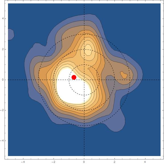
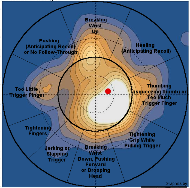
Although the mean is located 0.6 cm to the left of the center, shots are slightly to the lower left cuadrant. I'm a lefty, so my defect would be the equivalent to shooting down and to the right for a right handed person.

Let's see what the marksmanship tutorial chart has to say about this issue. enter image description here

I'm tightening the grip too hard while pulling the trigger. Will need to work on this more.

Now, what is the probability that I would hit the center within a radius of 0.5,1, 2 and 3.5 cm?

NProbability[
   EuclideanDistance[{0, 0}, {x, y}] <= #, {x, y} \[Distributed] kde, 
   PrecisionGoal -> 5] & /@ {0.5, 1, 2,3.5}
(*{0.0349262, 0.139871, 0.491972, 0.856485}*)

Given that an commercial apple is about 7cm in diameter. I've got a 86% chance of hitting it from a distance of 10 yards.

POSTED BY: Diego Zviovich
8 Replies
Posted 8 years ago

Hi Sjoerd, I've only shown one of the targets. There are seven targets that were scanned and used to create the distribution.

files = FileNames[
   "C:\\Users\\Diego\\Documents\\Documents\\Shooting\\10 yds\\scan*.jpg"];
imgs = Import[#] & /@ files;
Export["pics.png", Rasterize[Multicolumn[imgs, 4], 600]]

enter image description here

173 shots in total are used for the calculation of the distribution. Let's overlap all the shots on top of the first image.

s = Flatten[shots[#, kern] & /@ imgs, 1];
Length@s
(*173*)
centers = findCenter[#, kern] & /@ imgs;
Show[imgs[[1]],  Graphics[{Yellow, EdgeForm[Blue], 
   Disk[100 # + centers[[1]], 10] & /@ s}]];
Export["160513.png", Show[imgs[[1]],   Graphics[{Yellow, EdgeForm[Blue], 
Disk[100 # + centers[[1]], 10] & /@ s}], ImageSize ->  400]]

enter image description here

We can overlay the 173 shots against the contourplot. The contourplot now makes more sense.

Show[ContourPlot[PDF[kde, {x, y}], {x, -5, 5}, {y, -5, 5}], 
Graphics[{Dashed, Line[{{0, -5}, {0, 5}}], Line[{{-5, 0}, {5, 0}}], 
Circle[{0, 0}, #] & /@ {1, 2, 3}, Red, PointSize[0.03], 
Point@Mean@kde, Black, PointSize[0.01], Point[results]}], 
ImageSize -> Large, PlotTheme -> "Detailed"]

enter image description here

POSTED BY: Diego Zviovich

This is a really nice plot, but there is one thing that I don't really get: why is the DensityPlot the brightest in the lower-left quadrant even though by far the most shots landed in the upper-right one (8, compared to only 3 in the lower-left)? Are you sure you didn't flip the data somewhere in the code?

POSTED BY: Sjoerd Smit

enter image description here - another post of yours has been selected for the Staff Picks group, congratulations !

We are happy to see you at the tops of the "Featured Contributor" board. Thank you for your wonderful contributions, and please keep them coming!

POSTED BY: Moderation Team

Nice post! Instead of finding Mean you could try local maxima. Also there are many ways of overlapping images, like ImageMultiply or Overlay.

tutorial = Import["https://wolfr.am/cEj2VscY"];
heatmap = Import["https://wolfr.am/cEj0rqGj"];
cropT = ImageResize[ImageTake[tutorial, {100, 765}, {1, 665}], 600];
cropH = ImageReflect[ImageResize[ImageTake[heatmap, {10, 550}, {25, 570}], 610], Left -> Right];
ImageMultiply[cropH, cropT]

enter image description here

POSTED BY: Vitaliy Kaurov

Because of Diego's self-proclaimed left-handedness we have to reflect the density plot accordingly. Or come up with a left handed version of the shooting-diagnosis breakdown stencil.

POSTED BY: Anton Antonov

True! I did not notice his lefty comment. I corrected with ImageReflect, thanks.

POSTED BY: Vitaliy Kaurov

I still have a lot to learn... Awesome work!

Really interesting -- thanks for sharing!

Do you have timestamps associated with the shooting images? It would be interesting to do temporal-spatial mining of shooting performance.

Another set of data and questions come from the idea to cross-correlate with the traffic landscapes while driving to the shooting range.

POSTED BY: Anton Antonov
Reply to this discussion
Community posts can be styled and formatted using the Markdown syntax.
Reply Preview
Attachments
Remove
or Discard

Group Abstract Group Abstract