I liked Bret Victor's first example best because he turned a static paper into a dynamic paper with far more explanation of the topic and at least one illustration had a slider. The circuit example was more a design tool. In practice it would have to have much more support and documentation. The Jerome Bruner idea of Interactive-Visual-Symbolic (or numerical), that is combining them, is a very good principle of dynamic presentations. The introduction of the Playfair plot on trade balances should remind us that types of presentations that we now take for granted had to be invented. Mathematica gives us a fantastic new palette of tools to convey information. Nevertheless, these are relatively new and it's going to take a lot of experimentation and practice to learn how to best use them. For example, just having a lot of things that move around can end up being quite confusing. Bret's difference equation is again a design tool. It seems to put the user in a restricted box. The polygon example was difficult for me to follow because he was trying to explain too many things in too short a time.
Another thing I liked a lot about Bret's presentation is that a number of the examples had a very nice free form and quite appropriate composition. He mixed graphics, dynamics, text and code just as if he was writing on a sheet of paper. I wish Mathematica had more of a paradigm for this. Mathematica's composition is rather chunky and clunky.
Another feature that Bret Victor had was the invisible slider to vary a displayed number. Does anyone know how to do this in Mathematica?
If you look up Bret Victor on YouTube, there are quite a few of his videos. Another one that I liked, which was a larger picture, was "The Human Representation of Thought".
There is, by the way, a rich history of innovators concerned with human-machine interaction who have brought us to where we are. Much of it is chronicled in Walter Isaacson's The Inovators. But, alas, the index doesn't even mention Mathematica, Wolfram, Adobe, LaTex or Knuth. Technical publication doesn't make the cut.
What I care about here is the Wolfram Language, Mathematica and applications as a publication medium. Almost everything is there. There is only one problem. As a medium for communicating information, it and others such as Bret Victor have competition. That competition is the millennia old, static written paper with textual discussion, equations and diagrams, and its offshoot, the nearly static PDF document. Static documents are winning hands down. Why? Maybe because it seems too difficult and maybe because most users don't see examples. Few are done. The nearest thing is the Demonstration project, which are good practice and exploration of dynamic techniques. But they don't raise to the level of extended publications.
So, as an example, I thought I would post snapshots of a notebook that might raise to the level of a publication and using the active and dynamic features of the Wolfram Language. The notebook concerns the fact that orbits in the Schwarzschild geometry in general relative can be calculated exactly using the Weierstrass Elliptic function. This seemed to have been only realized in this century and I only found out about it from Ron Burns, a retired physicist who was using some of my packages, and who sent me a short notebook on it, doing the calculation for Mercury and a pulsar. I found it so interesting that I decided to turn it into a longer tutorial and learn some of the features of elliptic functions, of which I had little knowledge. It also serves as a good example of why a Wolfram Language publication supported by applications is far superior to static printed publications.
Here is a screen shot of the beginning of the notebook. The first thing to notice is that it's supported by two applications: a UnitsHelper application that was used to introduce reduced geometric units, and the Presentations application that helped me custom design dynamic displays. The more usual case might be that the author might have his own application supporting the general subject matter and it might be used for a number of papers.
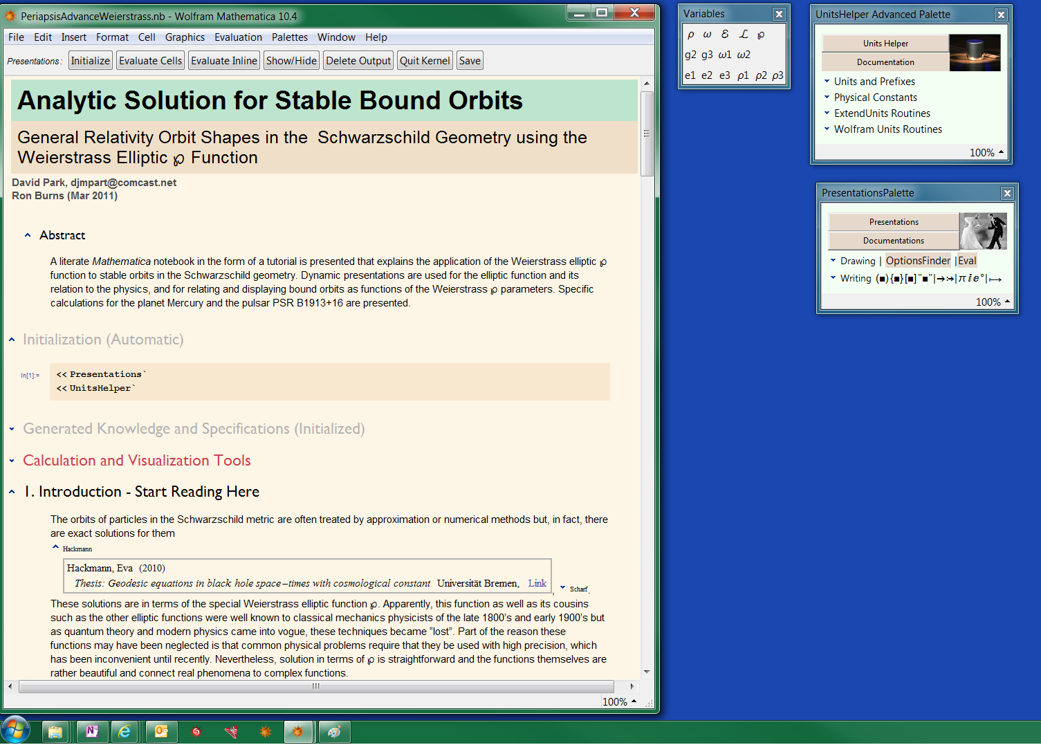
The reader, having Mathematica, can of course do the calculations in the notebook and can also try his own calculations. So there is a small paste palette for the most common symbols in the theory. There are also palettes that go with the supporting applications and the notebook uses a Stylesheet from one of them. The ability to actively calculate can eliminate many errors and typos that plague static printed papers. It's still possible to make errors but the overall integrity of a notebook is much higher than a static paper. In this notebook there are inline references using openers that give the details and links to web documents when they exist.
In the Introduction to the Weierstrass function there is a Crib Sheet that gives the main definitions and identities of the function.
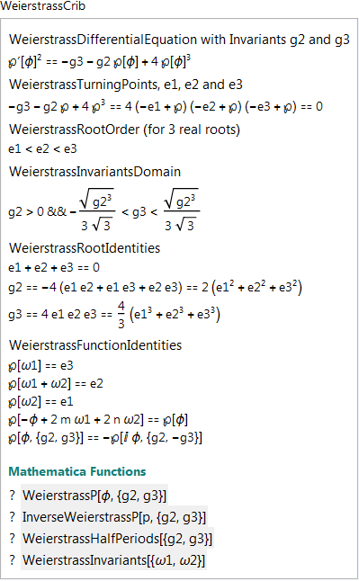
The Crib Sheet is launched as a side window. The various formulas can be pasted into a notebook. At the bottom of the Crib Sheet there are template paste buttons for the relevant Weierstrass functions and links to their help pages.
One feature I often use in notebooks is to write a specification for a graphic or dynamic display just where it is used in a notebook but then (semi) permanently close the cell. To notify the reader that the cell has to be evaluated I place an Eval button in the text cell preceding the display cell. The Eval button has a tooltip telling its purpose and also how the closed cell could be opened. And it's easier to click the Eval button than to fish for the closed cell bracket.
I also sometimes use cell buttons that give the user the choice of generating a predefined display in the notebook or as a side window. The advantage of side windows is that if there is extensive discussion in the notebook then the display won't scroll out of view.
There is a fair amount of calculation in the notebook demonstrating the properties of the WeierstrassP function and its physical application, which I'm not showing here. Rather I'm showing the features a notebook has over a static publication. The following dynamic display shows how the WeierstrassP Function tiles the complex plane. The function is defined by two parameters, g2 and g3. The graphic on the left shows the domain that gives real turning point values (e1, e2, e3), that correspond to real trajectories. The red points show the poles of the function. The green points show the turning points in one cell. The top of the tile plot is graduated in terms of 2 Pi and you can see that the real part of the elliptic period is different.
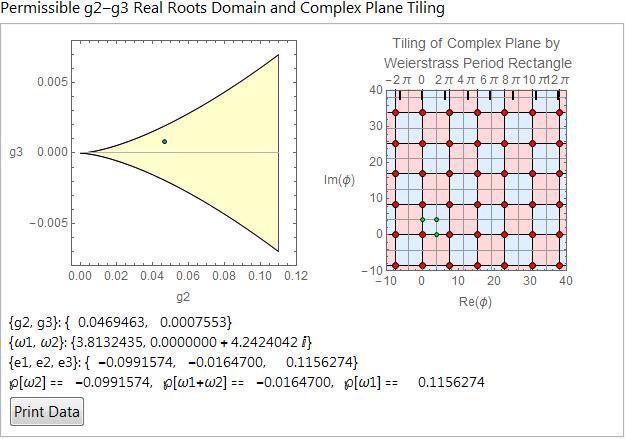
The display also illustrates the technique of combining dynamic graphics with numerical or symbolic data. Here we can print the data into a notebook as an Association. Associations are a very nice feature of Mathematica because, among other things, they provide context for the numbers.
<|"g2" -> 0.0469463, "g3" -> 0.000755332, "\[Omega]1" -> 3.81324,
 "\[Omega]2" -> 0. + 4.2424 I, "\[ScriptCapitalE]" -> 1.04526,
 "\[ScriptCapitalL]" -> 5.24236, "e1" -> -0.0991574, "e2" -> -0.01647,
  "e3" -> 0.115627, "\[Rho]1" -> -31.5974, "\[Rho]2" -> 7.47793,
 "\[Rho]3" -> 2.51306|>
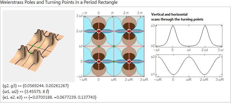
Another view of the WeierstrassP function is given by showing a surface plot of the real value along with a matching contour plot and scans through the horizontal and vertical turning points. The surface plot is rotatable and the contour plot is well annotated with tooltips. This also reminds us that Mathematica notebooks can freely use color, which is rare and expensive in printed papers. Also printed articles usually have page charges whereas notebooks can be longer without extra monetary expense. You are freer to explain in more detail when you think it is useful.
Getting to the physics, the supporting UnitsHelper application allows us to use geometric units where the gravitational constant and speed of light are taken as equal to 1.
SetupReducedUnits[{Quantity[1, "SpeedOfLight"],
  Quantity[1, "GravitationalConstant"]}, {Quantity["Meters"],
  Quantity["Amperes"], Quantity["Kelvin"]}]
{"Kilograms" -> 7.43*10^-28 "Meters", "Seconds" -> 299792458 "Meters"}
A key part of the tutorial is the transformation of the geodesic equation in the Schwarzschild metric (taken from a text) to the differential equation that defines the WeierstrassP function.
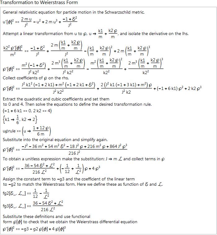
In that derivation there are tooltips on each expression showing the Wolfram Language expression that produced it. We can finally get to calculating and plotting some orbits.
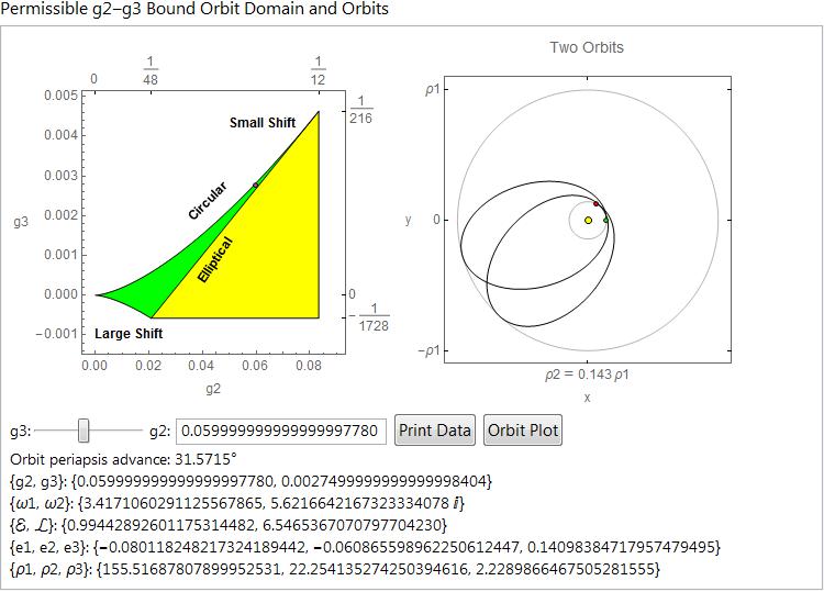
The green section of the g2-g3 domain is the region that gives bound orbits.The upper edge gives circular orbits and the lower edge gives highly elliptical orbits, so elliptical that they look like a ticking hand of a clock. All the perihelion advancement is near the center. A red locator can be moved to select a domain point but there is a problem because the green region becomes a narrow slice at the upper right and that's where many interesting physical cases occur. However, extra precision is used in the dynamic and the g3 slider automatically puts the locator within the thin slice. This is a case where the dynamic presentation must be adapted to the particular conditions of the case. I usually use a DynamicModule for these displays because they give me greater ability to control the composition of the display.
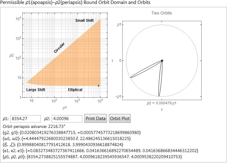
There is also a similar domain-orbit dynamic using the radial turning points of an orbit. The green locator can be used to pick the radial parameters, or they can be entered in the InputFields. Here a highly elliptical orbit is shown.
The orbits are determined by two parameters but there are choices of which two parameters are used. The user is provided by a routine that allows any pair of parameters and returns all parameters as an Association
step1 = AllOrbitParameters[\[Omega]1\[Omega]2][4.7, 5.5 I]
Inactivate[
 AllOrbitParameters[\[ScriptCapitalE]\[ScriptCapitalL]] @@ ({"\
\[ScriptCapitalE]", "\[ScriptCapitalL]"} /. step1), AllOrbitParameters]
Activate[%]
giving
<|"g2" -> 0.0192086, "g3" -> 0.000276706, "\[Omega]1" -> 4.7,
 "\[Omega]2" -> 0. + 5.5 I, "\[ScriptCapitalE]" -> 0.968605,
 "\[ScriptCapitalL]" -> 3.949, "e1" -> -0.0604853, "e2" -> -0.0151259,
  "e3" -> 0.0756112, "\[Rho]1" -> 21.8837, "\[Rho]2" -> 7.33058,
 "\[Rho]3" -> 3.14575|>
 AllOrbitParameters][\[ScriptCapitalE]\[ScriptCapitalL][0.968605, 3.949]
<|"g2" -> 0.0192086, "g3" -> 0.000276706, "\[Omega]1" -> 4.7,
 "\[Omega]2" -> 0. + 5.5 I, "\[ScriptCapitalE]" -> 0.968605,
 "\[ScriptCapitalL]" -> 3.949, "e1" -> -0.0604853, "e2" -> -0.0151259,
  "e3" -> 0.0756112, "\[Rho]1" -> 21.8837, "\[Rho]2" -> 7.33058,
 "\[Rho]3" -> 3.14575|>
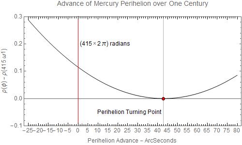
Extracting the data for the planet Mercury from NASA or Wikipedia, which the inline references link to, and skipping some of the notebook calculations we finally calculate the difference between the WeierstrassP real half period and a regular orbit half period to get the perihelion advance per orbit. Multiplying by the number of orbits in a century we obtain the result that gave Einstein heart palpitations.
2 (\[Omega]1Mercury - \[Pi]) Quantity[1, "Radians"]/orbit;
% 415 orbit // ToUnit[Quantity[1, "ArcSeconds"]];
NumberForm[%, {5, 3}]
giving
42.958"
And, using high precision, plot the radial function around the century mark.
Let's look at the advantages.
1) You are handing the reader a document with supporting routines that allow him to quickly perform the calculations himself and extend or modify them.
2) You can provide the reader with multiple forms of presentation including graphics, dynamic presentations or step by step derivations and proofs. In other words, something like a classic paper but with active and dynamic features added.
3) Since calculations and dynamics must work, this produces a higher integrity document. It doesn't eliminate all possibility of error but certainly reduces the probability. Often an error first becomes manifest in a graphic or dynamic display. Edward Tufte writes (in Visual Explanations) "Those who discover an explanation are often those who construct its representation." Publishing with notebooks will encourage a variety of presentations and the attendant exploration and discoveries.
4) Readers can more easily respond with additions, suggestions or criticisms using the tools you've handed them.
5) If the paper is within an application the reader could even add his own package and maybe share routines and results with you.
6) You can use color and longer documents freely.
Wolfram could do many things to improve and smooth their product for this usage. But basically the technology is here. Why aren't you using it?


