Message Boards Message Boards

[Challenge] The Pink Triangle Problem

I just came across a puzzle on phys.org, which apparently went viral on Twitter. Ed Southall posted a question regarding a problem about the area of a triangle. We are asked what fraction of the area the pink triangle occupies:

enter image description here

It is quite easy to find the answer. What is more interesting is to find as many ways as possible for that. On MentalFloss they describe some approaches to solve the puzzle. The main idea of the "classical solutions" presented on that website are based on the similarity of triangles. I was wondering what computational thinking and the Wolfram Language could do for us...

Setting the problem up

It is necessary to "interpret the sketch". For example, we need to recognise that we can choose the base to be of length one, and that the other two sides have slope 2 and -1. With that we can define the region like so:

reg = ImplicitRegion[2 x >= y && y <= 1 - x && 0 <= x <= 1 && 0 <= y <= 1, {x, y}];

I generated the plot above with this function:

RegionPlot[reg, PlotRange -> {{0, 1}, {0, 1}}, PlotStyle -> RGBColor[1, .1, 1], FrameTicks -> False]

enter image description here

Stephen Wolfram often says that the Wolfram Language is very useful also to state problems (read his blog posts on AI and on communicating with aliens). This becomes quite clear here. The definition of the ImplicitRegion makes the problem very clear; in fact much more precise than the image alone!

Solution 1

The easiest solution is now to ask Mathematica directly for the answer:

Area[reg]

which gives 1/3 as expected.

Solution 2

We can also use a Monte Carlo approach and generate points in the unit square and see how many of them are in the "pink region":

M = 1000000; N[Length[Select[RandomPoint[Rectangle[{0, 0}, {1, 1}], M], 2 #[[1]] >= #[[2]] && #[[2]] <= 1 - #[[1]] &]]/M]

which obviously gives slightly different results every time you run it. I got 0.333633 which is quite close to 1/3.

Solution 3

The problem with the previous solution is that it is numerical and only gives an approximate value. The Wolfram Language also allows us to use the distributions to effectively run a Monte Carlo simulation on an "infinite number of points".

dist = UniformDistribution[{{0, 1}, {0, 1}}];
Probability[2 x >= y \[And] y <= 1 - x, {x, y} \[Distributed] dist]

which results in 1/3, so the precise result.

Solution 4

If we recognise that in the definition of the implicit region defines the region by using the equations of two straight lines

y==2 x && y == 1 - x 

We can then calculate where they intersect, i.e. the tip of the triangle:

sols = Solve[y == 2 x && y == 1 - x, {x, y}]

This gives

{{x -> 1/3, y -> 2/3}}

Where y is the height of the triangle. So then the area of the pink triangle is

area=1/2 (x*y) + 1/2 ((1 - x)*y) /. sols[[1]]

This come uses the hight line to calculate the areas of the resulting "left and right triangle". It is easier of course because we know that the length of the base of the triangle is 1 and the height is y so that we can write:

area = y/2

(Just simplify the previous equation to get to this result!)

As y is 2/3 we obtain 1/3 for the area of the pink triangle again.

Solution 5

This one is going to be nice. We first import the image from the phys.org website:

img = Import["https://3c1703fe8d.site.internapcdn.net/newman/gfx/news/2018/5ae713bf2d29a.jpg"];

You will notice that around the black square there is a slim white border, which can be removed using ImageCrop. There are three colours in the remaining plot: white, pink and black. We can ignore the black points (as they are only lines, i.e. one dimensional). The two dominating colours will be white and pink. So lets take all pixels and find three clusters of the values, corresponding to white, pink and black:

clusters = FindClusters[Flatten[ImageData[ImageCrop[img]], 1], 3];

We now need to count how many points/pixels we have in any cluster. Then we will sort the sizes, and ignore the smallest one (i.e. black). Then we compute the ratio of pink points to all points:

N[#[[2]]/Total[#[[{2, 3}]]]] &@Sort[Length /@ clusters]

which gives 0.333709, so a very good approximate value.

Conclusion

You will notice that some of the solutions are distinctly different from the analytical and geometrical approaches presented on the mental floss website. I would classify the approaches I describe here as rather "computational" approaches. I challenge you to find further computational approaches and see what we can contribute to the discussion on twitter.

POSTED BY: Marco Thiel
11 Replies

Hi,

Simplifying the use of regions and avoiding the need to describe the lines, I thought this was quite accessible to school students: Define two shapes:

tri1 = Triangle[{{0, 0}, {0, 2}, {2, 0}}/2];poly = Polygon[{{0, 0}, {1, 2}, {2, 2}, {2, 0}}/2];

Visualise:

Graphics[{Opacity[0.2], Red, tri1, poly}, Frame -> True]

enter image description here

Do an intersection to find the original pink triangle:

reg = RegionIntersection[tri1, poly]

Visualise and compute the area:

{Region[reg], Area[reg]}
POSTED BY: Alec Titterton

You are missing the obvious Integrate, which could be done even without a Piecewise function:

Integrate[Min[2 x, 1 - x], {x, 0, 1}]

1 / 3

Or this:

Integrate[1, {x, y} \[Element] reg]

Cheers,

Marco

POSTED BY: Marco Thiel

Here is something different (and a bit flawed): Let's try machine learning.

  1. First we generate a training set:

    training = 
      ParallelTable[{\[Alpha], \[Beta]} = {RandomReal[{0, 5}], 
         1}; \[Gamma] = RandomReal[{0, 1}]; 
       reg = ImplicitRegion[\[Alpha] x >= y && y <= 1 - \[Beta] x && 
          0 <= x <= 1 && 0 <= y <= 1, {x, y}]; 
       RegionPlot[reg, PlotRange -> {{0, 1}, {0, 1}}, 
         PlotStyle -> RGBColor[
          0.9960635289608001, 0.12544040437828788`, 0.9997459270575916], 
         FrameTicks -> False, ImageSize -> 100] -> Area[reg], {k, 200}];
    
  2. Then we train a predictor:

    predictArea = Predict[training]
    
  3. Applying this to our original image gives:

    reg = ImplicitRegion[2 x >= y && y <= 1 - x && 0 <= x <= 1 && 0 <= y <= 1, {x, y}];
    img=RegionPlot[reg, PlotRange -> {{0, 1}, {0, 1}}, PlotStyle -> RGBColor[0.9960635289608001, 0.12544040437828788`, 0.9997459270575916], FrameTicks -> False];
    predictArea[ImageResize[img,100]]
    

which, in my case, gave: 0.328286.

Cheers,

Marco

POSTED BY: Marco Thiel

In terms of "computational" we could try to make Ed's proof into a little interactive experience (the video is too fast, but you can easily try the code below!):
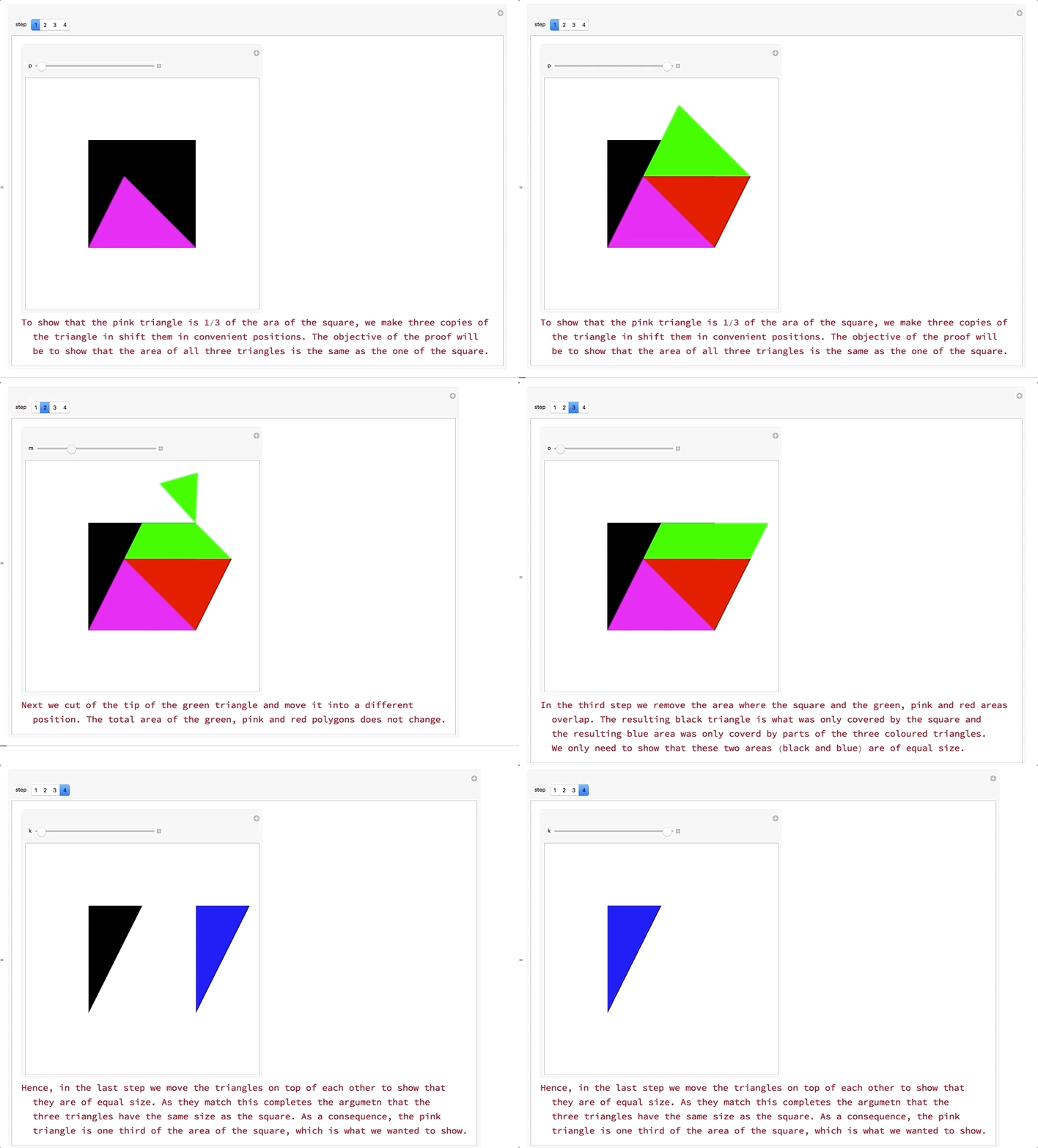
enter image description here

You need to work your way through steps one to 4 and always move the slider appropriately from left to right.

(*From the documentation*)
SymmetricSubdivision[Triangle[pl_], k_] /; 0 <= k < 2^Length[pl] :=
 Module[{n = Length[pl] - 1, i0, bl, pos},
  i0 = DigitCount[k, 2, 1]; bl = IntegerDigits[k, 2, n];
  pos = FoldList[If[#2 == 0, #1 + {0, 1}, #1 + {1, 0}] &, {0, i0}, 
    Reverse[bl]];
  Triangle@Map[Mean, Extract[pl, #] & /@ Map[{#} &, pos + 1, {2}]] 
  ]

(*The magic Manipulate*)

Manipulate[
 Which[step == 1, 
  Column[{Manipulate[
     Graphics[{Rectangle[{0, 0}, {1, 1}], RGBColor[
       0.9960635289608001, 0.12544040437828788`, 0.9997459270575916], 
       Triangle[{{0, 0}, {1, 0}, {1/3, 2/3}}], 
       Blend[{RGBColor[
         0.9960635289608001, 0.12544040437828788`, 
          0.9997459270575916], Green}, p], 
       Triangle[{{0, 0} + p {1/3, 2/3}, {1, 0} + 
          p {1/3, 2/3}, {1/3, 2/3} + p {1/3, 2/3}}], 
       Blend[{RGBColor[
         0.9960635289608001, 0.12544040437828788`, 
          0.9997459270575916], Red}, p], 
       Translate[
        GeometricTransformation[
         Triangle[{{0, 0}, {1, 0}, {1/3, 2/3}}], 
         RotationTransform[Pi p]], p {1 + 1/3, 2/3}]}, 
      PlotRange -> {{-0.5, 1.5}, {-0.5, 1.5}}], {p, 0, 1}], 
    Style["To show that the pink triangle is 1/3 of the area of the \
square, we make three copies of the triangle in shift them in \
convenient positions. The objective of the proof will be to show that \
the area of all three triangles is the same as the one of the \
square.", 15, Red]}], step == 2, 
  Column[{Manipulate[
     Graphics[{Rectangle[{0, 0}, {1, 1}], RGBColor[
       0.9960635289608001, 0.12544040437828788`, 0.9997459270575916], 
       Triangle[{{0, 0}, {1, 0}, {1/3, 2/3}}], 
       Green, {GeometricTransformation[#[[4]], 
           RotationTransform[-m Pi, {1, 
             1}]], #[[1]], #[[2]], #[[3]]} &@(SymmetricSubdivision[
            Triangle[{{0, 0} + {1/3, 2/3}, {1, 0} + {1/3, 2/3}, {1/3, 
                2/3} + {1/3, 2/3}}], #] & /@ Range[0, 3]), Red, 
       Translate[
        GeometricTransformation[
         Triangle[{{0, 0}, {1, 0}, {1/3, 2/3}}], 
         RotationTransform[Pi ]], {1 + 1/3, 2/3}]}, 
      PlotRange -> {{-0.5, 1.5}, {-0.5, 1.5}}], {m, 0, 1}], 
    Style["Next we cut of the tip of the green triangle and move it \
into a different position. The total area of the green, pink and red \
polygons does not change.", 15, Red]}], step == 3, 
  Column[{Manipulate[
     Graphics[{Opacity[o], Rectangle[{0, 0}, {1, 1}], RGBColor[
       0.9960635289608001, 0.12544040437828788`, 0.9997459270575916], 
       Triangle[{{0, 0}, {1, 0}, {1/3, 2/3}}], 
       Green, {GeometricTransformation[#[[4]], 
           RotationTransform[- Pi, {1, 
             1}]], #[[1]], #[[2]], #[[3]]} &@(SymmetricSubdivision[
            Triangle[{{0, 0} + {1/3, 2/3}, {1, 0} + {1/3, 2/3}, {1/3, 
                2/3} + {1/3, 2/3}}], #] & /@ Range[0, 3]), Red, 
       Translate[
        GeometricTransformation[
         Triangle[{{0, 0}, {1, 0}, {1/3, 2/3}}], 
         RotationTransform[Pi ]], {1 + 1/3, 2/3}], Opacity[1 - o], 
       Black, Triangle[{{0, 0}, {1/2, 1}, {0, 1}}], Blue, 
       Triangle[{{1, 0}, {1 + 1/2, 1}, {1, 1}}]}, 
      PlotRange -> {{-0.5, 1.5}, {-0.5, 1.5}}], {o, 1, 0}], 
    Style["In the third step we remove the area where the square and \
the green, pink and red areas overlap. The resulting black triangle \
is what was only covered by the square and the resulting blue area \
was only coverd by parts of the three coloured triangles. We only \
need to show that these two areas (black and blue) are of equal \
size.", 15, Red]}], step == 4, 
  Column[{Manipulate[
     Graphics[{Triangle[{{0, 0}, {1/2, 1}, {0, 1}}], Blue, 
       Triangle[{{1, 0} - k {1, 0}, {1 + 1/2, 1} - k {1, 0}, {1, 1} - 
          k {1, 0}}]}, PlotRange -> {{-0.5, 1.5}, {-0.5, 1.5}}], {k, 
      0, 1}], Style[
     "Hence, in the last step we move the triangles on top of each \
other to show that they are of equal size. As they match this \
completes the argument that the three triangles have the same size as \
the square. As a consequence, the pink triangle is one third of the \
area of the square, which is what we wanted to show.", 15, 
     Red]}]], {step, {1, 2, 3, 4}}]

This is still not computational thinking but it might help students/pupils to better grasp the idea of the proof that Ed has described.

I'd love to hear your comments.

Cheers,

Marco

PS: Notebook attached.

Attachments:
POSTED BY: Marco Thiel

enter image description here - Congratulations! This post is now a Staff Pick as distinguished by a badge on your profile! Thank you, keep it coming!

POSTED BY: EDITORIAL BOARD

@Marco, I just wanted to say how cool this idea is in terms of demonstrating the educational value of computational thinking. Even in this simple example it enables people to explore the problem in much wider context. This in turn brings much better understanding of the problem itself and educates people about new extravagant to the problem fields such as probability or image processing. And you actually wrote it so very neatly in the form of Computational Essay. Kudos and thanks!

POSTED BY: Vitaliy Kaurov

Dear @Vitaliy Kaurov,

yes, it is indeed something similar to a Computational Essay. I have been playing around with that type of approach even for pre-school education. The computational thinking approach is somehow different from the typical mathematical thinking approach, but it is hard for me to nicely distinguish them, because the transition is a bit fluid, which is of course wanted. It might be artificial to distinguish these problem solving techniques.

The computational approach seems to allow users to look at the problem from many different angles and finally help them to develop a mathematical proof, with or without computer assistance. It would be nice to see how future automatic proof structures in the Wolfram Langauge will blur the distinction even more.

I have been thinking of how to use FindEquationalProof to find another solution for this particular problem. FindGeometricalProof would be really cool of course.

Best wishes,

Marco

POSTED BY: Marco Thiel

Another image processing approach would be getting at a binarized image:

i = Binarize[RegionPlot[reg, PlotRange -> {{0, 1}, {0, 1}}, Frame -> False]]

enter image description here

and the using ImageMeasurements:

ImageMeasurements[i, "Total"]/Times @@ ImageDimensions[i]

0.3388888888888889

POSTED BY: Vitaliy Kaurov

A visual proof is also possible.

p = {{0, 0}, {1, 0}, {1/3, 2/3}, {4/3, 2/3}, {2/3, 4/3}, {0, 0}, {0, 1}, {1/2, 1}, {1, 1}, {1, 0}, {4/3, 2/3}};
up = Union[p];
char = Characters["ABCDEFGH"];
Graphics[{Line[p], Line[{{1/3, 2/3}, {0, 1}}], Table[Style[Text[char[[n]], up[[n]]] , 30], {n, 1, 8}]}]

enter image description here

If you need the proof spelled out,
Triangle ACF=HFC=CEH
Triangle ABC=FGH
Triangle BCD=GED

POSTED BY: Ed Pegg

Dear Ed,

thank you for your proof. Yes, that is indeed a typical way to mathematically prove that the area is one third and it is a very nice representation with Mathematica. I would consider this to be a mathematical/analytical solution. You need to think like a mathematician to write down something like that.

I was wondering which "computational thinking"-type ways the Wolfram Language offers to answer the same question, but without needing mathematical intuition, but rather some computational approach.

I am not even sure whether that question makes sense, because I am not quite able to define "mathematical/analytical" approach vs "computational thinking" approach. The latter one might be more experimental if that makes sense.

I think that Stephen Wolfram has been talking about extensions of FindEquationalProof, which will work for geometrical objects. There was also a session on Twitch he posted, which talked about that. To some extent that would be interesting, and in particular I would not know whether that would be a computational (i.e. CAS system) or a mathematical (,i.e. requires mathematical thinking) proof. The boundaries are somehow melting away...

Thank you very much again.

Best wishes,

Marco

POSTED BY: Marco Thiel
Reply to this discussion
Community posts can be styled and formatted using the Markdown syntax.
Reply Preview
Attachments
Remove
or Discard

Group Abstract Group Abstract