Message Boards Message Boards

1
|
5880 Views
|
4 Replies
|
6 Total Likes
View groups...
Share
Share this post:

Color Gradients Across a Circle

Posted 11 years ago
Hi All,

I would like to make a Disk with more than one color on it. Right now I've got:
n = 100;
Graphics[Table[{ColorData["GrayYellowTones"][i/n],
   Disk[{0, 0}, (i/n + .5)]}, {i, n, 1, -1}]]
which produces the following image . I would like to do this in a smarter way so I don't have to draw loads of circles.

Any suggestions? Thanks!
POSTED BY: Cesar Sul
4 Replies
There is no way that doesn't use lots of graphics primitives.

Instead of using disks, you can build it from polygons in a simple way using something like:
DensityPlot[Sqrt[x^2 + y^2], {x, -1, 1}, {y, -1, 1},
RegionFunction -> Function[{x, y}, x^2 + y^2 < 1],
ColorFunction -> "Mint"]

You can visualize the polygons by adding the option Mesh -> All and you can control how many there will be using PlotPoints and MaxRecursion.

One reason why it's necessary to have lots of polygons, and e.g. constructing the disk from "slices of pie" won't work well, is that a triangle Polygon[] can only interpolate linearly between the colours assigned to its vertices.  If you need a colour function which goes through several colours, e.g. Blend[{Red,Blue, Green, Orange}, #]&, then it's necessary to have enough subdivision so all the intermediate colours will have a chance to appear.

If you change Mint to Rainbow above, you'll be able to see what I'm talking about: the structure of the underlying grid will be visible because there isn't enough granularity to smoothly go through all the colours in this colour function.  You'll need to increase the PlotPoints to get a smooth look.
POSTED BY: Szabolcs Horvát
Here is another way:

PieChart[{1}, ChartElementFunction -> ChartElementData["GradientSector", "ColorScheme" -> "GrayYellowTones", "GradientDirection" -> "Radial"]]
POSTED BY: Vitaliy Kaurov
Hi Cesar,

this is not elegant, but the problem is that Disk does apparently not allow for textures. But this works: 
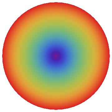
img = Rasterize[
  DensityPlot[x, {x, -4, 4}, {y, -4, 4}, ColorFunction -> "Rainbow",
   Frame -> False, PlotRangePadding -> None]];

ParametricPlot[{r*Cos[t], r*Sin[t]}, {r, 0, 1}, {t, 0, 2 Pi},
Mesh -> False, BoundaryStyle -> None, Axes -> False, Frame -> False,
PlotStyle -> {Opacity[1], Texture[img]}]

This is the result:


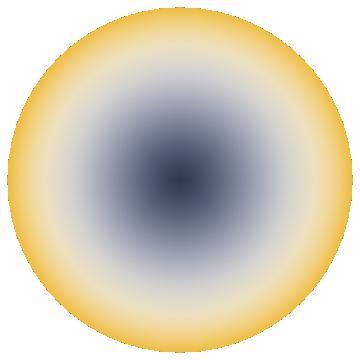
The code is longer than yours, but this allows easily to use any image as texture and the idea is quite simple. If you use yellowtones instead it looks like that:


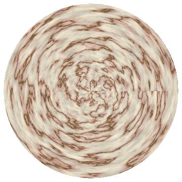
With other textures one can get:
ParametricPlot[{r*Cos[t], r*Sin[t]}, {r, 0, 1}, {t, 0, 2 Pi},
Mesh -> False, BoundaryStyle -> None, Axes -> False, Frame -> False,
PlotStyle -> {Opacity[1],
   Texture[ExampleData[{"ColorTexture", "WhiteMarble"}]]}]


M.
POSTED BY: Marco Thiel
It is actually quite interesting. Mathematica is really flexible. The different pieces of code in the question and in all three replies tell the same story but with very different words! Beautiful, isn't it?

M. 
POSTED BY: Marco Thiel
Reply to this discussion
Community posts can be styled and formatted using the Markdown syntax.
Reply Preview
Attachments
Remove
or Discard

Group Abstract Group Abstract