
The excellent community contribution by @Greg Hurst and a Wikipedia animation, Inspired me to look further into this "rolling shutter effect on rotating objects". When we capture a video of a rotating disk with a rolling shutter, we have two independent movements: the colored disk rotating at rps revolutions per second and the shutter line sweeping one frame at fps frames per second. The ratio rps/fps is the driver of the rolling shutter effect (or the disk rps alone if we normalize the shutter fps to 1 frame per second). In order to best demonstrate this effect, ratios of rps/fps are taken to be in the range 1.5-2.5
This is a colored disk of m pixels wide, rotated over an angle theta.
colors = {RGBColor[1, 0, 1], RGBColor[0.988, 0.73, 0.0195], RGBColor[
   0.266, 0.516, 0.9576], RGBColor[0.207, 0.652, 0.324], RGBColor[
   0, 0, 1], RGBColor[1, 0, 0]};
colorDisk[theta_, m_, cols_] :=
 ImageResize[
  Image[Graphics[
    MapThread[{#3,
       Disk[{0, 0}, 1, {#1, #2} + theta]} &, {Pi Range[0, 5, 1]/3,
      Pi Range[1, 6]/3, colors}]]], m]
A video of the rotating disk consists of a series of frames. Each frame is captured during one passage of the shutter line. The function angularPosition links the angular progress of the disk to the frame number (frm) and the row number at the position of the shutter line:
angularPosition[frm_, row_, rps_,
  m_] := -2 Pi (-1 + (-1 + frm) m + row) rps/m
Th function diskFrameImage computes the result of the shutter line swiping a colored disk (of size m, rotating at rps revolutions per second) at frame number frm and up to row number toRow:
diskFrameImage[frm_, toRow_, rps_, m_, cols_] :=
 ImageAssemble[
  Transpose@{ParallelTable[
     ImageTake[
      colorDisk[angularPosition[frm, r, rps, m], m, colors], {r}], {r,
       toRow}]}]
This is the first frame of a video of a disk rotating at a speed ratio rps/fps of 1 :
With[{m = 200, frm = 1, rps = 1},
 diskFrameImage[frm, m, rps, m, colors]]

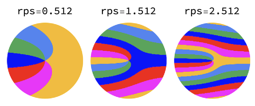
This shows the influence of the disk rps/fps ratio on the appearance of the first frame captured:
With[{m = 200, frm = 1},
 Grid[{{"rps=0.512", "rps=1.512", "rps=2.512"},
   diskFrameImage[frm, m, #, m, colors] & /@ {.512, 1.512, 2.512}}]]
Below is a GIF showing the capture of the first frame of a disk rotating at rps/fps 1. The code is used to generate all of the following GIFs.
With[{m = 200, frm = 1, rps = 1.},
 Animate[
  Grid[{{
     ImageCompose[
      colorDisk[angularPosition[frm, row, rps, m], m, colors],
      Graphics[Line[{{-m, 0}, {m, 0}}]], Scaled[{.5, (m - row)/m}]],
     ImageCompose[diskFrameImage[frm, row, rps, m, colors],
      Graphics[Line[{{-m, 0}, {m, 0}}]], Scaled[{.5, .01}]]}},
   Alignment -> Top], {row, 1, m}]]

Below are 4 examples showing the capture of the first frame of a video of a rotating disk with a roller shutter at 1fs. The disk rotates at 0.5 rps (top left), 1.0 rps (top right), 1.5 rps (bottom left) and 2.0 rps (bottom right). As the disk rotates faster relative to the shutter, the captured image becomes more complex.


The subsequent frames are captured the same way. Below are the first 5 frames of a video of a disk rotating at 1.5123 rps:
There ought to be a lot more images that result from the transformation of a rotation into a capture with a rolling shutter. I hope this contribution can inspire more community members.


