Message Boards Message Boards

Imaging a rotating disk with a rolling shutter

Posted 2 years ago

enter image description here

The excellent community contribution by @Greg Hurst and a Wikipedia animation, Inspired me to look further into this "rolling shutter effect on rotating objects". When we capture a video of a rotating disk with a rolling shutter, we have two independent movements: the colored disk rotating at rps revolutions per second and the shutter line sweeping one frame at fps frames per second. The ratio rps/fps is the driver of the rolling shutter effect (or the disk rps alone if we normalize the shutter fps to 1 frame per second). In order to best demonstrate this effect, ratios of rps/fps are taken to be in the range 1.5-2.5

This is a colored disk of m pixels wide, rotated over an angle theta.

colors = {RGBColor[1, 0, 1], RGBColor[0.988, 0.73, 0.0195], RGBColor[
   0.266, 0.516, 0.9576], RGBColor[0.207, 0.652, 0.324], RGBColor[
   0, 0, 1], RGBColor[1, 0, 0]};
colorDisk[theta_, m_, cols_] := 
 ImageResize[
  Image[Graphics[
    MapThread[{#3, 
       Disk[{0, 0}, 1, {#1, #2} + theta]} &, {Pi Range[0, 5, 1]/3, 
      Pi Range[1, 6]/3, colors}]]], m]

A video of the rotating disk consists of a series of frames. Each frame is captured during one passage of the shutter line. The function angularPosition links the angular progress of the disk to the frame number (frm) and the row number at the position of the shutter line:

angularPosition[frm_, row_, rps_, 
  m_] := -2 Pi (-1 + (-1 + frm) m + row) rps/m

Th function diskFrameImage computes the result of the shutter line swiping a colored disk (of size m, rotating at rps revolutions per second) at frame number frm and up to row number toRow:

diskFrameImage[frm_, toRow_, rps_, m_, cols_] := 
 ImageAssemble[
  Transpose@{ParallelTable[
     ImageTake[
      colorDisk[angularPosition[frm, r, rps, m], m, colors], {r}], {r,
       toRow}]}]

This is the first frame of a video of a disk rotating at a speed ratio rps/fps of 1 :

With[{m = 200, frm = 1, rps = 1}, 
 diskFrameImage[frm, m, rps, m, colors]]

enter image description here

This shows the influence of the disk rps/fps ratio on the appearance of the first frame captured:

With[{m = 200, frm = 1}, 
 Grid[{{"rps=0.512", "rps=1.512", "rps=2.512"}, 
   diskFrameImage[frm, m, #, m, colors] & /@ {.512, 1.512, 2.512}}]]
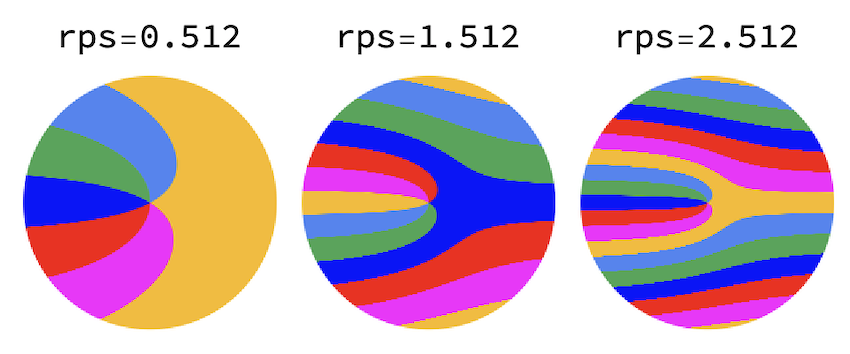
enter image description here

Below is a GIF showing the capture of the first frame of a disk rotating at rps/fps 1. The code is used to generate all of the following GIFs.

With[{m = 200, frm = 1, rps = 1.},
 Animate[
  Grid[{{
     ImageCompose[
      colorDisk[angularPosition[frm, row, rps, m], m, colors], 
      Graphics[Line[{{-m, 0}, {m, 0}}]], Scaled[{.5, (m - row)/m}]],
     ImageCompose[diskFrameImage[frm, row, rps, m, colors], 
      Graphics[Line[{{-m, 0}, {m, 0}}]], Scaled[{.5, .01}]]}}, 
   Alignment -> Top], {row, 1, m}]]

enter image description here

Below are 4 examples showing the capture of the first frame of a video of a rotating disk with a roller shutter at 1fs. The disk rotates at 0.5 rps (top left), 1.0 rps (top right), 1.5 rps (bottom left) and 2.0 rps (bottom right). As the disk rotates faster relative to the shutter, the captured image becomes more complex.

enter image description here

enter image description here

The subsequent frames are captured the same way. Below are the first 5 frames of a video of a disk rotating at 1.5123 rps:
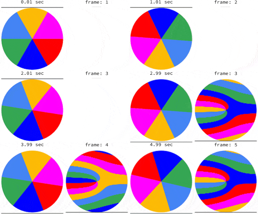
enter image description here

There ought to be a lot more images that result from the transformation of a rotation into a capture with a rolling shutter. I hope this contribution can inspire more community members.

POSTED BY: Erik Mahieu
14 Replies

We now have a collection of creative post about “Rolling Shutter”. Here is the full current list for them:

Airplane propellers imaged with a rolling shutter
https://community.wolfram.com/groups/-/m/t/2489445

Rolling Shutter III
https://community.wolfram.com/groups/-/m/t/2543358

Modeling the Rolling Shutter Effect
https://community.wolfram.com/groups/-/m/t/2809149

POSTED BY: EDITORIAL BOARD
Posted 2 years ago

Thanks for pointing that out. Should be fixed now.

POSTED BY: Greg Hurst
Posted 2 years ago

I believe there is a very minor typo: the flag should read: PlotStyle -> Texture[texture] ?

POSTED BY: c pichon

Thanks, Greg, for doing the Riemann sphere... a nice addition to this already colorful thread.

It's possible (probable?) that the visual similarity arises from expansions around a zero being dominated by low-order linear terms.

But what I was really hoping for may be too unrealistic--Is there a description of something like the Eisenstein series in terms of rotating propellers and sliding shutters?

POSTED BY: Brad Klee
Posted 2 years ago

I think this might just be a characteristic of plotting in the complex plane. Take a look at https://community.wolfram.com/groups/-/m/t/2543358.

In these type of plots, zeros, poles, and essential singularities are illustrated quite nicely here.

enter image description here

This particular function has a zero at the origin and an essential singularity at infinity, shown by the white arrows:

f[z_?NumericQ] := Exp[I (2.25 Im[z])] z

ComplexPlot[f[z], {z, 2}, ColorFunction -> "CyclicArg"]

The essential singularity can be seen on the Riemann sphere. Below, the south pole shows the zero at the origin and the north pole shows the essential singularity at infinity.

plot = ComplexPlot[f[Tan[Im[z]/2] Exp[I*Re[z]]], {z, -π, π + π*I}, ColorFunction -> "CyclicArg", RasterSize -> 2048];

texture = ImageResize[Cases[plot, _Image, ∞][[1]], Scaled[{1, 1/2}]];

rsphere = SphericalPlot3D[1, {u, 0, π}, {v, -π, π}, Mesh -> None, 
  TextureCoordinateFunction -> ({#5, 1 - #4} &), 
  PlotStyle -> Texture[texture], Lighting -> "Neutral", Axes -> False, 
  PlotPoints -> 100, SphericalRegion -> True
];

South pole:

Show[rsphere, ViewPoint -> {-1.3, -2.4, 2.}, ViewVertical -> {0, 0, -1}]

North pole:

Show[rsphere, ViewPoint -> {1.3, 2.4, -2.}, ViewVertical -> {0, 0, 1}]

POSTED BY: Greg Hurst

Can anyone prove is this related at all to modular functions?

Compare with the following from wikipedia:

enter image description here

Modular functions are not that easy to understand, so a nice proof about how they could relate to this straightforward transformation construction would make this post even more interesting! It looks within reach...

POSTED BY: Brad Klee
Posted 2 years ago

Thanks equally for the suggestion.Here is Mona with two different speed ratios shutter vs image: 1.0 in the center and 2.0 at right:

enter image description here

Have fun!

POSTED BY: Erik Mahieu

Thanks for the suggestion. You could also make a weight lifter version of the Mona Lisa (apply it on the ImageTransformation sample image) =D

Posted 2 years ago

Looks like a good entry for the "Wolfram One -liner competition"! It also solves my problem to convert any image into a "roller shutter captured" image. here is the transformation on he Wolfram logo using your code:

enter image description here

POSTED BY: Erik Mahieu

You can use the following code to transform an image in one step:

ImageAdd[ImageTransformation[img, Block[{x, y}, {x, y} = #; 
    RotationTransform[(550 - y*550)*Degree, {.5, .5}][{x, y}]] &], 
 Graphics@Disk[]]

manipulate 550 for different options.

Example:

enter image description here

Posted 2 years ago

Nice piece of programming! Thanks Greg for your original "rolling shutter effect" idea.

POSTED BY: Erik Mahieu
Posted 2 years ago

And here's a way to do this with a continuous color wheel. This is sort of a blend between your idea and @Henrik Schachner's posted here.

The idea is with a standard color wheel we can exploit its cyclic nature and turn rotation into scalar addition. Just add a constant to the h channel to rotate the wheel.

hsbImage = Compile[{{r, _Integer}},
  Table[{(ArcTan[r - j - .001, i - r] + π)/(2π), 1, 1}, {i, 0, 2r}, {j, 0, 2r}]
];

r = 1024;
rps = 2.25;

base = Image[hsbImage[r], ColorSpace -> "HSB"];
mask = Image[DiskMatrix[r]];

splits = ImagePartition[base, {2r + 1, 1}][[All, 1]];

transform = ImageAssemble @ Table[
  {ImageAdd[splits[[k]], Hue[rps * k/(2r + 1), 0, 0]]}, 
  {k, 2r + 1}
];

Here we do a little trickery to renormalize the hues and turn the image into a disk:

final = ColorCombine[
  {
    ImageMultiply[Mod[#1, 1], mask], 
    ImageMultiply[#2, mask], 
    #3
  }& @@ ColorSeparate[transform], 
  "HSB"
]

To add discrete sectors, like in the original post above, we can simply round:

Round[final, 1/6]

POSTED BY: Greg Hurst
Posted 2 years ago

Great idea to vary the revolutions per second!

We can think of rps as the z-axis and visualize in 3D:

propeller[θ_] := Sin[3θ + π/2];

With[{r = Sqrt[x^2 + y^2], θ = ArcTan[x, y]},
  RegionPlot3D[
    r <= propeller[θ - π*z*x],
    {x, -1, 1}, {y, -1, 1}, {z, 0, 2.25},
    Frame -> None,
    PlotPoints -> 50 (* change to 100 or 200 if you're brave *)
  ]
]

enter image description here

POSTED BY: Greg Hurst

enter image description here -- you have earned Featured Contributor Badge enter image description here Your exceptional post has been selected for our editorial column Staff Picks http://wolfr.am/StaffPicks and Your Profile is now distinguished by a Featured Contributor Badge and is displayed on the Featured Contributor Board. Thank you!

POSTED BY: EDITORIAL BOARD
Reply to this discussion
Community posts can be styled and formatted using the Markdown syntax.
Reply Preview
Attachments
Remove
or Discard

Group Abstract Group Abstract