Thanks, Anton. I'm looking forward to the simulation. It would be interesting to model this as a first layer of the terraforming problem: how much forcing changes the surface conditions, and how quickly the system loses what it gains. The retention problem may be the harder part, so some kind of atmospheric protection, like the Mars-Sun L1 magnetic shield idea, seems relevant too.

@Vitaliy, this is actually nice to quickly draw different depths of the North Sea. In Aberdeen we are proceeding with what they call "energy transition". For example when they are looking for $CO_2$ storage sites there are many requirements, e.g. regarding the depth of the sea floor etc. With your code you can mark different depth ranges, e.g. in the North Sea from 80-100 m like so

(* =====North Sea+NE Atlantic:relief land,blue sea,80\[Dash]\
100m in red=====*)(*Region as {{latMin,latMax},{lonMin,lonMax}}.\
Extended N/NW so a genuine 3\[Dash]4 km depth band exists.*)
region = {{50, 70}, {-14, 16}};

(*Depth band to flag,in metres (negative=below sea surface).*)
{dDeep, dShallow} = {-100, -80};   (*sea floor 80-100m down*)

(*Land ramp:green lowland->tan->brown->white peaks (metres).*)
land[e_] := 
  Blend[{RGBColor[0.24, 0.45, 0.22], RGBColor[0.45, 0.55, 0.27], 
    RGBColor[0.75, 0.68, 0.42], RGBColor[0.52, 0.39, 0.26], White}, 
   Rescale[Clip[e, {0, 2500}], {0, 2500}]];

(*Sea ramp:pale shelf->deep blue (metres).*)
sea[e_] := 
  Blend[{RGBColor[0.78, 0.88, 0.96], RGBColor[0.30, 0.55, 0.80], 
    RGBColor[0.08, 0.25, 0.55], RGBColor[0.02, 0.08, 0.25]}, 
   Rescale[Clip[e, {-5000, 0}], {0, -5000}]];

(*Master colour function.\
Argument is elevation in METRES because ColorFunctionScaling->\
False below.\
QuantityMagnitude guards against the value arriving as a Quantity in s\
ome versions.*)
elevColor = 
  Function[e0, 
   With[{e = QuantityMagnitude[e0]}, 
    Which[e >= 0, land[e],(*land*)dDeep <= e <= dShallow, 
     Red,(*3\[Dash]4 km deep sea*)True, sea[e]     (*all other sea*)]]];

GeoGraphics[{}, GeoRange -> region, GeoProjection -> "Mercator", 
 GeoBackground -> 
  GeoStyling["ReliefMap", ColorFunction -> elevColor, 
   ColorFunctionScaling -> False], GeoGridLines -> Automatic, 
 ImageSize -> 850]

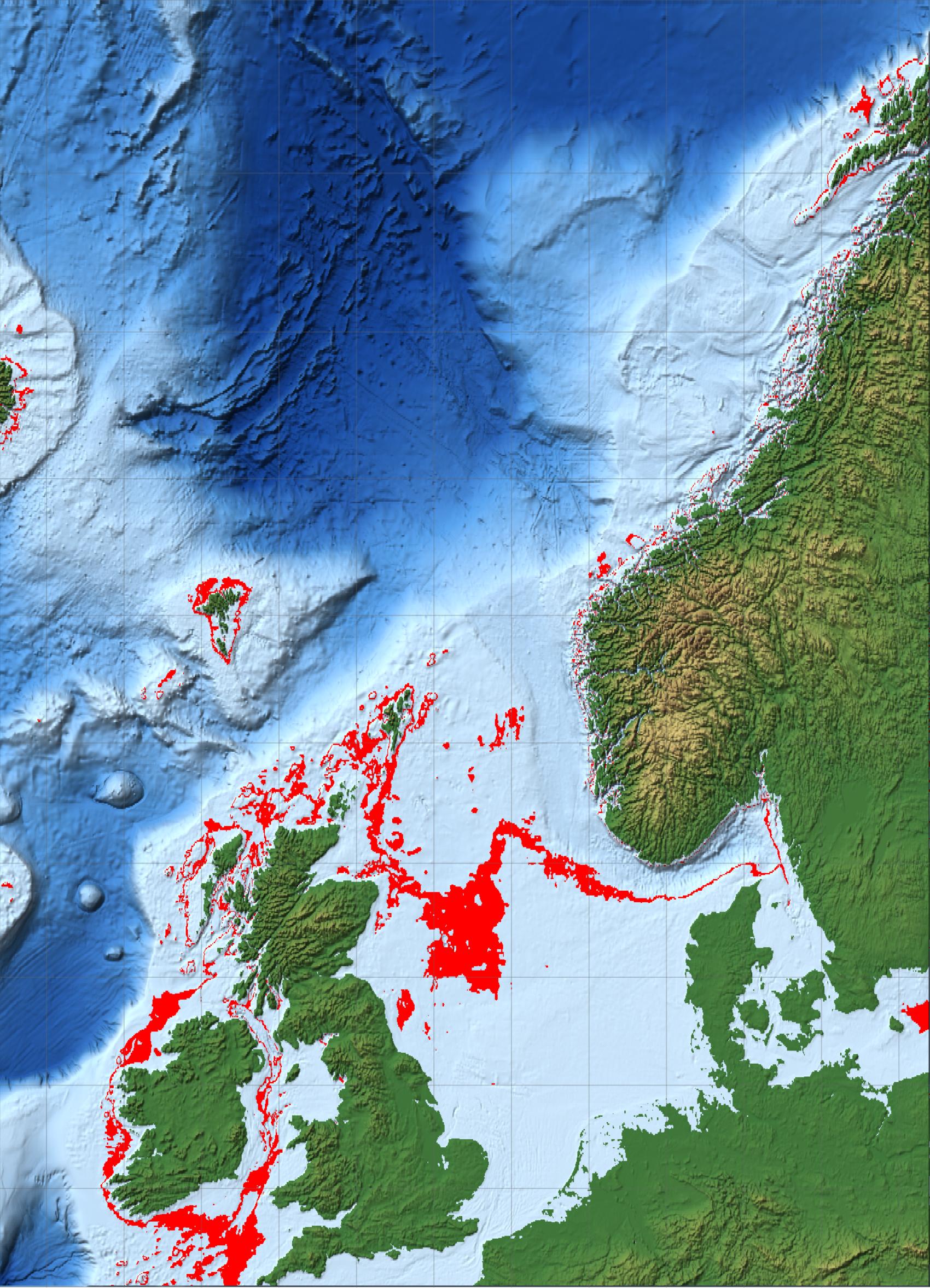
If you want to shade the different depths, that looks like this:

    (* =====North Sea+NE Atlantic:relief land,blue sea,80\[Dash]\
    100m in red=====*)(*Region as {{latMin,latMax},{lonMin,lonMax}}.\
    Extended N/NW so a genuine 3\[Dash]4 km depth band exists.*)
    region = {{50, 70}, {-14, 16}};

    (*Depth band to flag,in metres (negative=below sea surface).*)
    {dDeep, dShallow} = {-100, -80};   (*sea floor 80-100m down*)

    (*Land ramp:green lowland->tan->brown->white peaks (metres).*)
    land[e_] := 
      Blend[{RGBColor[0.24, 0.45, 0.22], RGBColor[0.45, 0.55, 0.27], 
        RGBColor[0.75, 0.68, 0.42], RGBColor[0.52, 0.39, 0.26], White}, 
       Rescale[Clip[e, {0, 2500}], {0, 2500}]];

    (*Sea ramp:pale shelf->deep blue (metres).*)
    sea[e_] := 
      Blend[{RGBColor[0.78, 0.88, 0.96], RGBColor[0.30, 0.55, 0.80], 
        RGBColor[0.08, 0.25, 0.55], RGBColor[0.02, 0.08, 0.25]}, 
       Rescale[Clip[e, {-5000, 0}], {0, -5000}]];

    (*Master colour function.\
    Argument is elevation in METRES because ColorFunctionScaling->\
    False below.\
    QuantityMagnitude guards against the value arriving as a Quantity in s\
    ome versions.*)
    elevColor = 
      Function[e0, 
       With[{e = QuantityMagnitude[e0]}, 
        Which[e >= 0, land[e],(*land*)dDeep <= e <= dShallow, 
         Red,(*3\[Dash]4 km deep sea*)True, sea[e]     (*all other sea*)]]];

    GeoGraphics[{}, GeoRange -> region, GeoProjection -> "Mercator", 
     GeoBackground -> 
      GeoStyling["ReliefMap", ColorFunction -> elevColor, 
       ColorFunctionScaling -> False], GeoGridLines -> Automatic, 
     ImageSize -> 850]


![enter image description here][2]

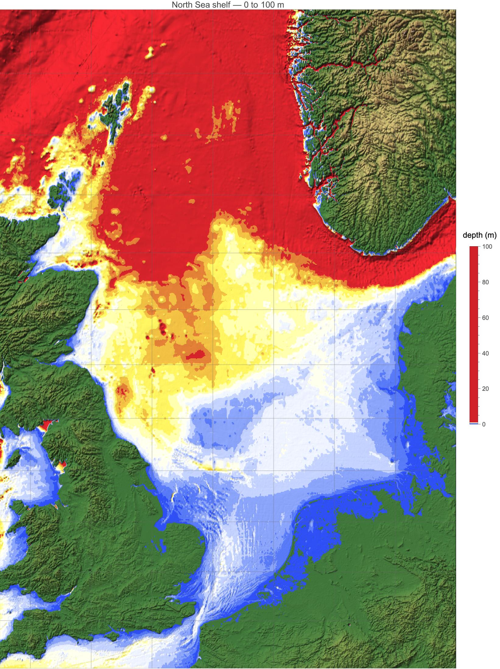
It turns out that the North Sea is really shallow....

(*North Sea shelf:sea floor 0 to-100 m,coloured by depth*)
region = {{50, 62}, {-5, 10}};         (*North Sea*)
dMax = 100;                           (*colour scale spans 0 to 100 m*)
step = 10;                            \
(*band thickness,m;set 0 for smooth*)
seaScheme = 
  ColorData[
   "TemperatureMap"];   \
(*or "Rainbow","DeepSeaColors","SouthwestColors"*)

land[e_] := 
  Blend[{RGBColor[0.24, 0.45, 0.22], RGBColor[0.45, 0.55, 0.27], 
    RGBColor[0.75, 0.68, 0.42], RGBColor[0.52, 0.39, 0.26], White}, 
   Rescale[Clip[e, {0, 2500}], {0, 2500}]];

depthColor = 
  Function[e0, 
   With[{e = QuantityMagnitude[e0]}, 
    If[e >= 0, land[e], 
     seaScheme[
      Clip[(If[step > 0, step*Floor[(-e)/step], -e])/dMax, {0, 1}]]]]];

Legended[
 GeoGraphics[{}, GeoRange -> region, GeoProjection -> "Mercator", 
  GeoBackground -> 
   GeoStyling["ReliefMap", ColorFunction -> depthColor, 
    ColorFunctionScaling -> False], GeoGridLines -> Automatic, 
  ImageSize -> 750, 
  PlotLabel -> Style["North Sea shelf \[LongDash] 0 to 100 m", 14]], 
 BarLegend[{seaScheme, {0, dMax}}, LegendLabel -> "depth (m)", 
  LegendMarkerSize -> 320]]

  [1]: https://community.wolfram.com//c/portal/getImageAttachment?filename=NorthSea80-100mdepth.jpg&userId=48754

Thanks Marco! Great images. What is the trick to build stylized exaggerated relief maps?

-- you have earned Featured Contributor Badge Your exceptional post has been selected for our editorial column Staff Picks http://wolfr.am/StaffPicks and Your Profile is now distinguished by a Featured Contributor Badge and is displayed on the Featured Contributor Board. Thank you!