Message Boards Message Boards

400th anniversary of Shakespeare's death

NOTE: the actual APP that does some analysis of Shakespeare's "Romeo and Juliet" is located HERE. Please wait through a potential little load or evaluation times, it is computing ! ;-) Read below and through comments for many ideas on Shakespeare's data mining.

enter image description here

I also highly recommend reading recent related blog by Jofre Espigule and checking out his Wolfram Cloud app that does some social and linguistic visualizations of the Shakespeare's texts:

enter image description here

April 23, 2016 marks 400th anniversary of Shakespeare’s death. Just a few decades of life's work produced texts that fascinate humanity for already 400 years. This centuries-old fascination tells us Shakespeare's works highlight the perpetual social and cultural phenomena. And also that Shakespeare is a seldom genius, a true master of the written and spoken word. But have you ever thought that Shakespeare's texts can be deemed as data? Perhaps Emerging filed of digital humanities can tell us what to read between the lines. Modern technologies can provide a new insight into social networks of characters, semantic, statistical and other properties of corpus that is usually considered of only high artistic value. Is there a pattern in the art?

Could you think of data mining analysis or visualizations to apply to Shakespeare's works? Please share your thoughts! Dive with Wolfram technologies into infinite depths of Shakespeare's data.

EXAMPLE: Storyline

Imagine I would like to see in a few quick pictures how the dramatic development of events propagates through a play. I consider "Romeo and Juliet" and download full text as a string (lower-casing all words):

romeojuliet = ToLowerCase[Import["http://shakespeare.mit.edu/romeo_juliet/full.html"]];

Now I will write a function drama that displays the density of a specific word in a play. It is done by indexing positions of words in the text and then running SmoothKernelDistribution algorithm hidden inside SmoothHistogram function that also plots the density:

drama[keywords_List] := With[
  {pos = StringPosition[romeojuliet, #][[All, 1]] & /@ keywords},
  SmoothHistogram[pos,
   Frame -> None, BaseStyle -> White,
   PlotLegends -> Placed[keywords, {{.93, .8}}],
   AspectRatio -> 1/3, ImageSize -> 700, PlotTheme -> "Marketing",
   PlotStyle -> {Automatic, Automatic, Dashed, Dashed, Dashed},
   Filling -> {1 -> {2}}, FillingStyle -> Directive[White, Opacity[.8]]]]

And now with a few computations drama reads the play and announces the verdict with just 3 images. Visually we see clearly what was important as the time went by. The 3rd image of interplay between "love", "hate", "life", and "death" speaks the most.

drama[{"romeo", "juliet", "life", "death"}]
drama[{"romeo", "juliet", "love", "hate"}]
drama[{"love", "hate", "life", "death"}]

enter image description here

To make a cloud app, we need to modify function a bit and use CloudDeploy.

dramaFORM[keywords_String] := Rasterize@Module[
   {pos, leg, keys = TextWords[ToLowerCase[keywords]]},
   leg = {"romeo", "juliet"}~Join~keys;
   pos = StringPosition[romeojuliet, #][[All, 1]] & /@ leg;
   SmoothHistogram[DeleteCases[pos, {} | {_Integer}],
    Frame -> None, PlotLegends -> Placed[leg, Bottom],
    AspectRatio -> 1/3, ImageSize -> 700, PlotTheme -> "Marketing",
    PlotStyle -> {Automatic, Automatic}~Join~Table[Dashed, {Length[leg] - 2}],
    Filling -> {1 -> {2}}, FillingStyle -> Directive[White, Opacity[.8]]]]

CloudDeploy[FormFunction[{
    "x" -> <|"Label" -> "", 
    "Interpreter"->"String",
    "Hint"->"hint: love, death",
    "Help"->Style["type Shakespeare's words separated by spaces or comma, be patient, wait, behold ;-)",Italic]|>}, 
    dramaFORM[#x]&,
    AppearanceRules-><|
    "Title" -> Grid[{{"Evolution of topics through Romeo & Juliet"},{Spacer[{10,5}]},{img}},Alignment->Center], 
    "Description" -> "DETAILS:  http://wolfr.am/RomeoJuliet "|>,
    FormTheme -> "Black"],
"RomeoAndJuliet",   
Permissions->"Public"]

EXAMPLE: Wordcloud

It is also interesting to know how modern society sees Shakespeare. The code below for the word cloud runs over Encyclopedia Britannica article about Shakespeare.

text=Import["http://www.britannica.com/print/article/537853"];
base[w_]:=With[{tmp=WordData[w,"BaseForm","List"]}, If[(Head[tmp]===Missing)||tmp==={},w,tmp[[1]]]];
SetAttributes[base,Listable];
tst=Quiet[base[TextWords[StringDelete[DeleteStopwords[ToLowerCase[text]],DigitCharacter..]]]];
blackLIST={"shakespeare","william","th","iii","iv","vi"};
WordCloud[DeleteCases[DeleteCases[tst,_First],Alternatives@@blackLIST],
    WordOrientation->{{-\[Pi]/4,\[Pi]/4}},AspectRatio->1/3,
    ScalingFunctions->(#^.01&),ImageSize->800]

enter image description here

DATA & CODE SOURCES:

POSTED BY: Vitaliy Kaurov
8 Replies

Here is my little contribution which is based on Chris Wilson's Wolfram Summer School side project about "Book Colors".

  • Gather a list of Color Names:

    colornames = {" alice blue ", " antique white ", " aqua ", " aquamarine ", " azure ", " beige ", " bisque ", " black ", " blanched almond ", " blue ", " blue violet ", " brown ", " burly wood ", " cadet blue ", " chartreuse ", " chocolate ", " coral ", " cornflower blue ", " cornsilk ", " crimson ", " cyan ", " dark blue ", " dark cyan ", " dark golden rod ", " dark gray ", " dark green ", " dark khaki ", " dark magenta ", " dark olive green ", " dark orange ", " dark orchid ", " dark red ", " dark salmon ", " dark sea green ", " dark slate blue ", " dark slate gray ", " dark turquoise ", " dark violet ", " deep pink ", " deep sky blue ", " dim gray ", " dodger blue ", " fire brick ", " floral white ", " forest green ", " fuchsia ", " gainsboro ", " ghost white ", " gold ", " golden rod ", " gray ", " green ", " green yellow ", " honey dew ", " hot pink ", " indian red ", " indigo ", " ivory ", " khaki ", " lavender ", " lavender blush ", " lawn green ", " lemon chiffon ", " light blue ", " light coral ", " light cyan ", " light gray ", " light green ", " light pink ", " light salmon ", " light sea green ", " light skyblue ", " light slate gray ", " light steel blue ", " light yellow ", " lime ", " lime green ", " linen ", " magenta ", " maroon ", " medium blue ", " medium orchid ", " medium purple ", " medium sea green ", " medium slate blue ", " medium spring green ", " mediumturquoise ", " medium violetred ", " midnight blue ", " mint cream ", " misty rose ", " moccasin ", " navajo white ", " navy ", " old lace ", " olive ", " olive drab ", " orange ", " orange red ", " orchid ", " pale golden rod ", " pale green ", " pale turquoise ", " pale violet red ", " papaya whip ", " peach puff ", " peru ", " pink ", " plum ", " powder blue ", " purple ", " red ", " rosy brown ", " royal blue ", " saddle brown ", " salmon ", " sandy brown ", " sea green ", " sea shell ", " sienna ", " silver ", " sky blue ", " slate blue ", " slate gray ", " snow ", " spring green ", " steel blue ", " teal ", " thistle ", " tomato ", " turquoise ", " violet ", " wheat ", " white ", " white smoke ", " yellow ", " yellow green "};
    
  • Use the color Interpreter to get them in the WL:

    colors = Interpreter["Color"][colornames]
    

colors

  • Make a PieChart of the StringCounts of these color names:

    Column@Table[
    link="http://shakespeare.mit.edu/"<>works<>"/full.html";
    text=ToLowerCase[Import[link]];
    PieChart[
    ParallelMap[StringCount[text,#]&,colornames],
    ChartStyle->colors,
    PlotLabel->Hyperlink[TextCases[text,"Line",1],link],
    LabelingFunction->"RadialCenter",
    ChartLabels->Placed[colornames,"RadialCallout"],
    ImageSize->600],
    {works,StringSplit[#,"/"][[-2]]&/@Import["http://shakespeare.mit.edu/","Hyperlinks"][[3;;-8]]}]
    

Enjoy!

Attachments:
POSTED BY: Bernat Espigulé

This is a fun analysis Bernat, but I worry about the colossal dominance of red! Is there really so much blood? This leads me to suspect we might be picking up the word red inside other words, murdered springs to mind!

Rather than count occurrence of the sequence "r e d", Mathematica lets us examine the characters around it. Presume that a colour is only intended if it doesn't follow or precede any other letters. We loose some good data (ie plurals like "reds"), but we filter out cases like "murdered" above.

colourOccuranceTable = ParallelTable[
    text = ToLowerCase[Import[ "http://shakespeare.mit.edu/" <> works <> "/full.html"]];
    Count[ Nor @@ LetterQ /@ # & /@
        Characters[ StringDrop[ StringCases[text, _ ~~ # ~~ _], {2, 1 + StringLength[#]}]]
        ,True] & /@ colornames
    ,{works, (StringSplit[#, "/"][[-2]] & /@ Import["http://shakespeare.mit.edu/", "Hyperlinks"][[3 ;; -8]])}];

We can then sum this data up over all the works, and compare it to your original analysis.

Comparison

Red is looking slightly less dominant!

POSTED BY: David Gathercole

You are completely right David! Somehow I assumed that was due to the domineering qualities of red:

Red - is a bold color that commands attention! Red gives the impression of seriousness and dignity, represents heat, fire and rage, it is known to escalate the body's metabolism. Red can also signify passion and love. Red promotes excitement and action. It is a bold color that signifies danger, which is why it's used on stop signs. Using too much red should be done with caution because of its domineering qualities. Red is the most powerful of colors. The Psychology of Color

Thanks for noticing it. I've just updated the color names above:

colornames = StringJoin[" ", #, " "] & /@ colornames;

Now it looks just right:

Colors Shakespeare

POSTED BY: Bernat Espigulé
Attachments:
POSTED BY: Marco Thiel

I took this opportunity to use the Wolfram Language on XML documents, specifically a TEI (http://www.tei-c.org) version of "The Tempest," which can be found at the University of Oxford Text Archive (http://ota.ox.ac.uk).

We start by importing the xml document as an XMLObject.

tempestxml = Import["http://ota.ox.ac.uk/text/5725.xml", "XMLObject"];

After exploring the document a little, I found that I could extract lines by a specific speaker with Cases. Here is how to get all the lines spoken by Prospero:

proslines = 
  Cases[tempestxml, XMLElement["sp", {}, {XMLElement["speaker", _, {"Pros."}], line_}] :> line, Infinity];

I made a WordCloud of those lines, only to discover that we lack Elizabethan stopwords:

WordCloud[DeleteStopwords@ToLowerCase@TextWords[StringRiffle[Flatten[proslines//.XMLElement[_,_,content_]:>content]]]]

First Prospero WordCloud

It's much more satisfying after a minor tweak:

WordCloud[DeleteCases[DeleteStopwords@ToLowerCase@TextWords[StringRiffle[Flatten[
    proslines //. XMLElement[_, _, content_] :> content]]], "thee" | "thou" | "thy"]]

Second Prospero WordCloud

Why limit ourselves to one character, though?

linesbychar = First@First@# -> Last /@ # & /@ GatherBy[Cases[tempestxml, 
    XMLElement["sp", {}, {XMLElement["speaker", _, {char_}], line_}] :> char -> line, Infinity], First]; 

Grid[Partition[Column@{First@#, WordCloud[DeleteCases[DeleteStopwords@ToLowerCase@TextWords[
               StringRiffle[Flatten[Last@# //. XMLElement[_, _, content_] :> content]]], 
                    "thee" | "thou" | "thy"]]} & /@ linesbychar, 6], Frame -> All, Alignment -> Left]

WordClouds for all characters

We don't have to limit ourselves to characters, we can make WordCloud for each scene. In this document, each scene is contained in a <div>

scenes = Cases[tempestxml, XMLElement["div", _, div_] :> div, Infinity];
Grid[Partition[Column[{First@#, WordCloud[DeleteCases[DeleteStopwords@ToLowerCase@TextWords[
           StringRiffle[Flatten[Cases[Last@#, XMLElement["ab", _, line_] :> line, Infinity] //. XMLElement[_, _, content_] :> content]]],
             "thee" | "thou" | "thy"]]}] & /@ ((Replace[Flatten[Cases[#, 
                XMLElement["head", _, h_] :> (h //. XMLElement[_, _, content_] :> content)]], {s_String} :> s] -> Rest@#) & /@ scenes), 5],                 
                    Frame -> All, Alignment -> Left]

a WordCloud for each scene

POSTED BY: Aaron Enright
POSTED BY: Marco Thiel
Posted 9 years ago

@Marco Thiel , you are indeed fast. My take on the graph of characters, leaving the conversations between characters.

data = SemanticImport[
   "c:\\Users\\Diego\\Downloads\\will_play_text.csv", Automatic, 
   "Rows", Delimiters -> ";"];
data[[All, 
    4]] = (ToExpression@StringSplit[#, "."] & /@ 
     data[[All, 4]]) /. {} -> {Missing[Empty], Missing[Empty], 
     Missing[Empty]};
sentiment = 
  Classify["Sentiment", data[[All, 6]]] /. {"Neutral" -> 0, 
    "Positive" -> 1, "Negative" -> -1, Indeterminate -> 0};
data[[All, 6]] = Transpose[{data[[All, 6]], sentiment}];
ds = Dataset[
  AssociationThread[{"ID", "Play", "Phrase", "Act", "Scene", "Line", 
      "Character", "Text", "Sentiment"}, #] & /@ (Flatten /@ data)];
getEdges[play_, act_, scene_] := 
 DirectedEdge[#[[1]], #[[2]]] & /@ 
  Partition[
   ds[Select[#Play == play &] /* Union, {"Act", "Scene", "Phrase", 
       "Character"}][Select[#Act == act && #Scene == scene &], 
     "Character"] // Normal, 2, 1]
getGraph[play_] := 
 Graph[Flatten[
   getEdges[#[[1]], #[[2]], #[[3]]] & /@ (ds[
         Select[#Play == play &] /* Union, {"Play", "Act", "Scene"}] //
         Normal // Values // Most)], VertexLabels -> "Name", 
  ImageSize -> 1024]
getGraph["Othello"]

enter image description here

Well, what about how many movies or TV Shows were made of the most famous plays?

plays={"Macbeth", "Romeo and Juliet", "Othello", "Hamlet", "King Lear", \
"Richard III", "The Tempest", "Merry Wives of Windsor", "Titus \
Andronicus"}
movies[play_] := 
 Import["http://www.imdb.com/find?q=" ~~ 
    StringReplace[play, " " -> "%20"] ~~ 
    "&s=tt&exact=true&ref_=fn_tt_ex", "Data"][[4, 1]]

shakespeareMovies = {Length@movies[#], #} & /@ plays // Sort // 
   Transpose;
BarChart[#[[1]], BarOrigin -> Left, ChartLabels -> #[[2]], 
   Frame -> True, 
   PlotLabel -> "Shakespeare Based Movies"] &@shakespeareMovies

BarChart[#[[1]], BarOrigin -> Left, ChartLabels -> #[[2]], 
   Frame -> True, PlotLabel -> "Shakespeare Based Movies", 
   PlotTheme -> "Detailed", ImageSize -> Large] &@shakespeareMovies

enter image description here

POSTED BY: Diego Zviovich

Dear @Vitaliy Kaurov ,

I haven't had much time to do this but here are a couple of thoughts. It is certainly interesting to use the Wolfram Language to analyse Shakespeare's texts. He is very much on everyone's mind; here are the English language wikipedia requests:

data = WolframAlpha[ "Shakespeare", {{"PopularityPod:WikipediaStatsData", 1}, "ComputableData"}];
DateListPlot[data, PlotRange -> All, PlotTheme -> "Detailed", 
 AspectRatio -> 1/4, ImageSize -> 800, PlotLegends -> {"Shakespeare"},Filling -> Bottom]

enter image description here

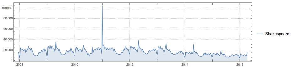
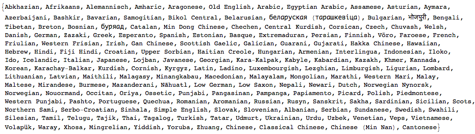
There is a clear peak every year on 23 April - the anniversary of his death. Of course, there are wikipedia articles in many other languages on Shakespeare:

WikipediaData["Shakespeare", "LanguagesList"]

enter image description here

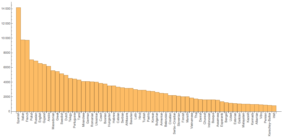
Interestingly, we can see the the longest articles are not (!) in English:

wikilength = 
  Select[{#, 
      Quiet[WordCount[
        WikipediaData[Entity["Person", "WilliamShakespeare::s9r82"], 
         "ArticlePlaintext", "Language" -> #]]]} & /@ 
    WikipediaData["Shakespeare", "LanguagesList"], NumberQ[#[[2]]] &];
BarChart[(Reverse@
    SortBy[Append[
      wikilength, {"English", 
       WordCount[
        WikipediaData[Entity["Person", "WilliamShakespeare::s9r82"], 
         "ArticlePlaintext"]]}], Last])[[1 ;; 60, 2]], 
 ChartLabels -> (Rotate[#, Pi/2] & /@ (Reverse@
      SortBy[Append[
         wikilength, {"English", 
          WordCount[
           WikipediaData[
            Entity["Person", "WilliamShakespeare::s9r82"], 
            "ArticlePlaintext"]]}], Last][[All, 1]]))]

enter image description here

I have downloaded the csv/xls version of the collected works you linked to, and then imported the data into Mathematica in the standard way:

texts = Import["/Users/thiel/Desktop/will_play_text.csv.xls"];

There are

Length[texts]

111396 rows in that file. They look like this:

texts[[1 ;; 10]] // TableForm

enter image description here

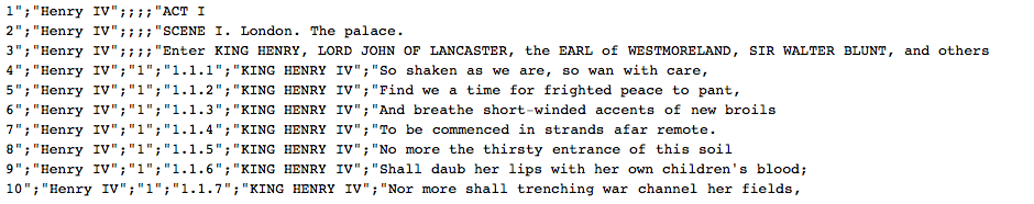
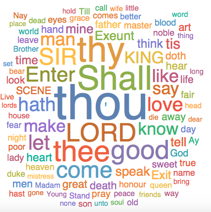
The first entry in every row just counts up then there is the name of the play, then two other bits of information on the position in the text, then there is the person who speaks and then there is what they say. There are also some spare quotation marks etc. This can be cleaned and we can look at the most important words that Shakespeare uses (here in his Sonnets):

WordCloud[
 DeleteStopwords[Flatten[TextWords /@ (StringReplace[StringSplit[#, ";"], "\"" -> ""] & /@ texts[[1 ;;, -1]])[[All, -1]]]], IgnoreCase -> True]

enter image description here

We can also count the words in all texts:

Length@Flatten[
  TextWords /@ (StringReplace[StringSplit[#, ";"], "\"" -> ""] & /@ texts[[1 ;;, -1]])[[All, -1]]]

which gives 775418 words. I can also sort the sentences by play like so

byplay = GroupBy[(StringReplace[StringSplit[#, ";"], "\"" -> ""] & /@ texts[[1 ;;, -1]]), #[[2]] &];

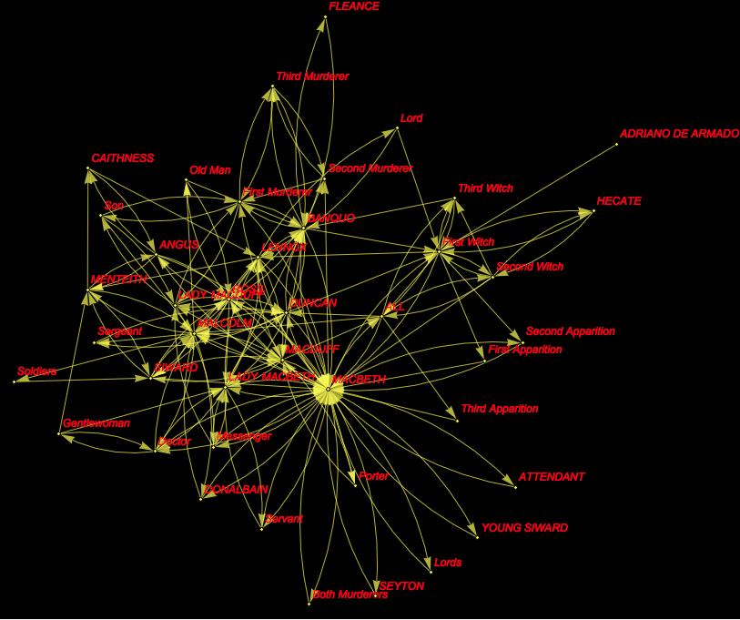
No magic here, but it is quite useful if we want to automatically generate a graph of who talks to whom, similar to one of the really cool demonstrations on the demonstration project:

g = Graph[
  DeleteDuplicates@(Rule @@@ 
     Partition[byplay[[18, All, 5]] //. {a___, x_, y_, b___} /; x == y -> {a, x, b}, 2, 1]), VertexLabels -> "Name", 
  VertexLabelStyle -> Directive[Red, Italic, 12], Background -> Black,EdgeStyle -> Yellow, VertexSize -> Small, VertexStyle -> Yellow]

byplay[[18, All, 5]] chooses play 18 - which happens to be Macbeth. It then takes all sentences and the speaker (entry 5). The rule deletes repeated speakers, i.e. if one speaker says several lines in a row I just use one incident. The Partition function always chooses two consecutive speakers (assuming that they interact). Finally I delete the duplicates and plot it; this give the following graph:

enter image description here

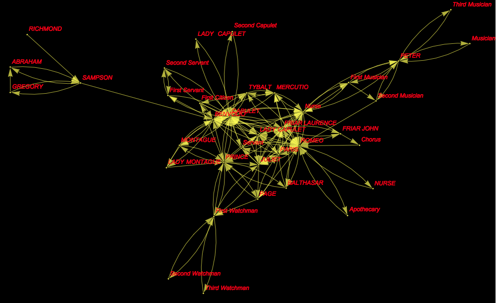
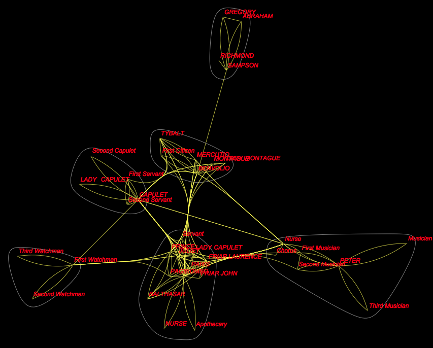
It is not trivial to make the same thing for other plays, say Romeo and Juliet (play 28):

g2 = Graph[
  DeleteDuplicates@(Rule @@@ 
     Partition[byplay[[28, All, 5]] //. {a___, x_, y_, b___} /; x == y -> {a, x, b}, 2, 1]), VertexLabels -> "Name", 
  VertexLabelStyle -> Directive[Red, Italic, 12], Background -> Black,EdgeStyle -> Yellow, VertexSize -> Small, VertexStyle -> Yellow]

enter image description here

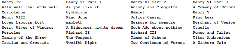
You can use the following to get a list of all plays:

Partition[Normal[byplay[[1 ;;, 1, 2]]][[All, 2]], 4] // TableForm

enter image description here

We can also use the very handy CommunityGraphPlot feature to look for groups of people in Romeo and Juliet:

g3 = CommunityGraphPlot[
  DeleteDuplicates@(Rule @@@ Partition[byplay[[28, All, 5]] //. {a___, x_, y_, b___} /; x == y -> {a, x, b}, 2, 1]), VertexLabels -> "Name", 
  VertexLabelStyle -> Directive[Red, Italic, 12], Background -> Black,EdgeStyle -> Yellow, VertexSize -> Small, VertexStyle -> Yellow]

enter image description here

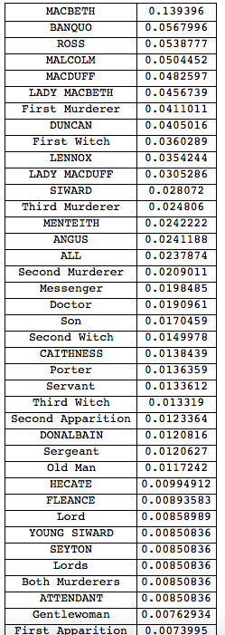
Oh, yes, and once we have the graphs we can use PageRank to figure out who the central characters are (for Macbeth):

Grid[Reverse@SortBy[Transpose[{VertexList[g], PageRankCentrality[g]}], Last], Frame -> All]

enter image description here

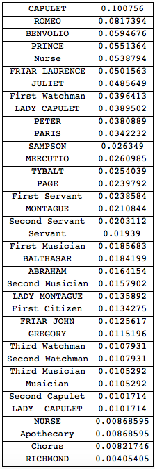
and here the same for Romeo and Juliet:

Grid[Reverse@SortBy[Transpose[{VertexList[g2], PageRankCentrality[g2]}], Last], Frame -> All]

enter image description here

Now I wanted to do something a bit more sophisticated, but the file I downloaded wasn't too good for that. I therefore downloaded the collection of all works of Shakespeare from the Gutenberg project:

shakespeare = Import["http://www.gutenberg.org/cache/epub/100/pg100.txt"];

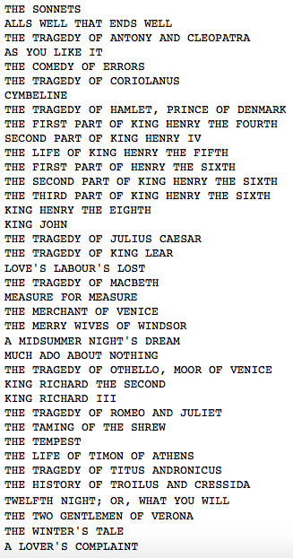
It contains the following titles:

titles = (StringSplit[#, "\n"] & /@ 
     StringTake[StringSplit[shakespeare, "by William Shakespeare"][[1 ;;]], -45])[[;; -3, -1]];
TableForm[titles]

enter image description here

It is all one long string, so we might want to split it into the different plays etc:

textssplit = (StringSplit[shakespeare, "by William Shakespeare"][[2 ;; -2]]);

I'll next delete a copyright comment and make a list of names of the plays and the corresponding texts.

alltexts = 
  Table[{titles[[i]], 
    StringDelete[textssplit[[i]], 
     "<<THIS ELECTRONIC VERSION OF THE COMPLETE WORKS OF WILLIAM
     SHAKESPEARE IS COPYRIGHT 1990-1993 BY WORLD LIBRARY, INC., AND 
     IS PROVIDED BY PROJECT GUTENBERG ETEXT OF ILLINOIS BENEDICTINE COLLEGE
     WITH PERMISSION.  ELECTRONIC AND MACHINE READABLE COPIES MAY BE
     DISTRIBUTED SO LONG AS SUCH COPIES (1) ARE FOR YOUR OR OTHERS
     PERSONAL USE ONLY, AND (2) ARE NOT DISTRIBUTED OR USED
     COMMERCIALLY.  PROHIBITED COMMERCIAL DISTRIBUTION INCLUDES BY ANY
     SERVICE THAT CHARGES FOR DOWNLOAD TIME OR FOR MEMBERSHIP.>>"]}, {i, 1, Length[titles]}];

Ok. Now we have something to work with. here is a primitive sentiment analysis, similar to the one we used for the GOP presidential debates.

sentiments = 
  Table[{titles[[i]], -"Negative" + "Positive" /. ((Classify["Sentiment", #, "Probabilities"] & /@ #) &@
       Select[TextSentences[alltexts[[i, 2]]], Length[TextWords[#]] > 1 &])}, {i, 1, Length[titles]}];

So we use a bit of machine learning and use the certainty of the algorithm to obtain estimates of sentiments. We should also average over a couple of consecutive sentences which is why we use MovingAverage

MovingAverage[sentiments[[4, 2]], 30] // ListLinePlot

enter image description here

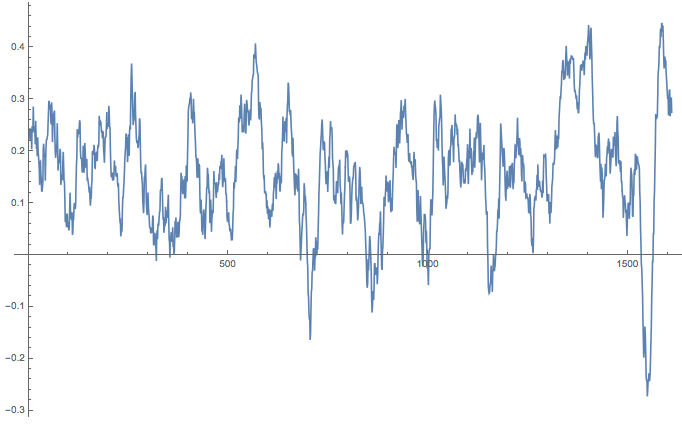
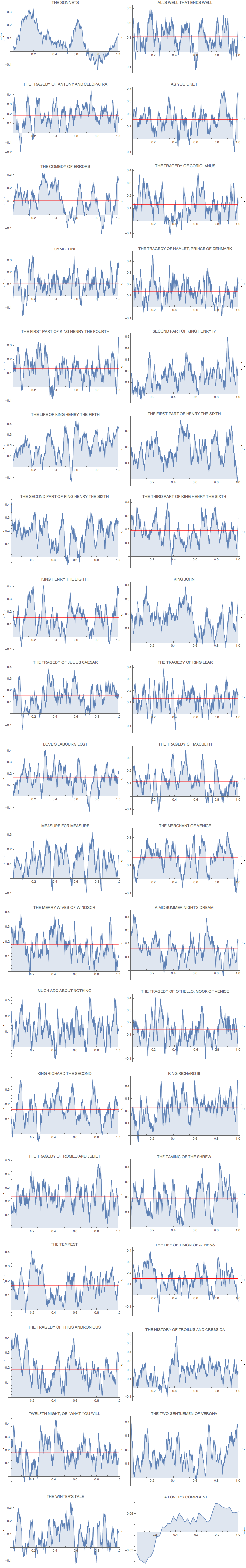
Ok. Let's normalise that to a standard length 1 (i.e. position in text in percent) and make it a bit more appealing:

ArrayReshape[
  ListLinePlot[
     Transpose@{Range[Length[#[[2]]]]/Length[#[[2]]], #[[2]]}, 
     PlotLabel -> #[[1]], Filling -> Axis, ImageSize -> Medium, 
     Epilog -> {Red, 
       Line[{{0, Mean[#[[2]]]}, {1, Mean[#[[2]]]}}]}] & /@ 
   Transpose@{titles, 
     MovingAverage[#, 50] & /@ sentiments[[All, 2]]}, {19, 
   2}] // TableForm

enter image description here

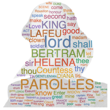
Let's make a couple of WordClouds for the individual plays. First I want an image of Shakespeare:

img = Import[
  "http://i0.wp.com/whatson.london/images/2013/07/Shakespeare.png?w=590"]; mask = Binarize[img, 0.0001];

We can then calculate a WordCloud in the shape of Shakespeare and overlay that to the image of the genius:

cloud = Image[WordCloud[DeleteStopwords[TextWords[alltexts[[2, 2]]]], mask, IgnoreCase -> True]]; 
ImageCompose[cloud, {ImageResize[img, ImageDimensions[cloud]], 0.2}]

enter image description here

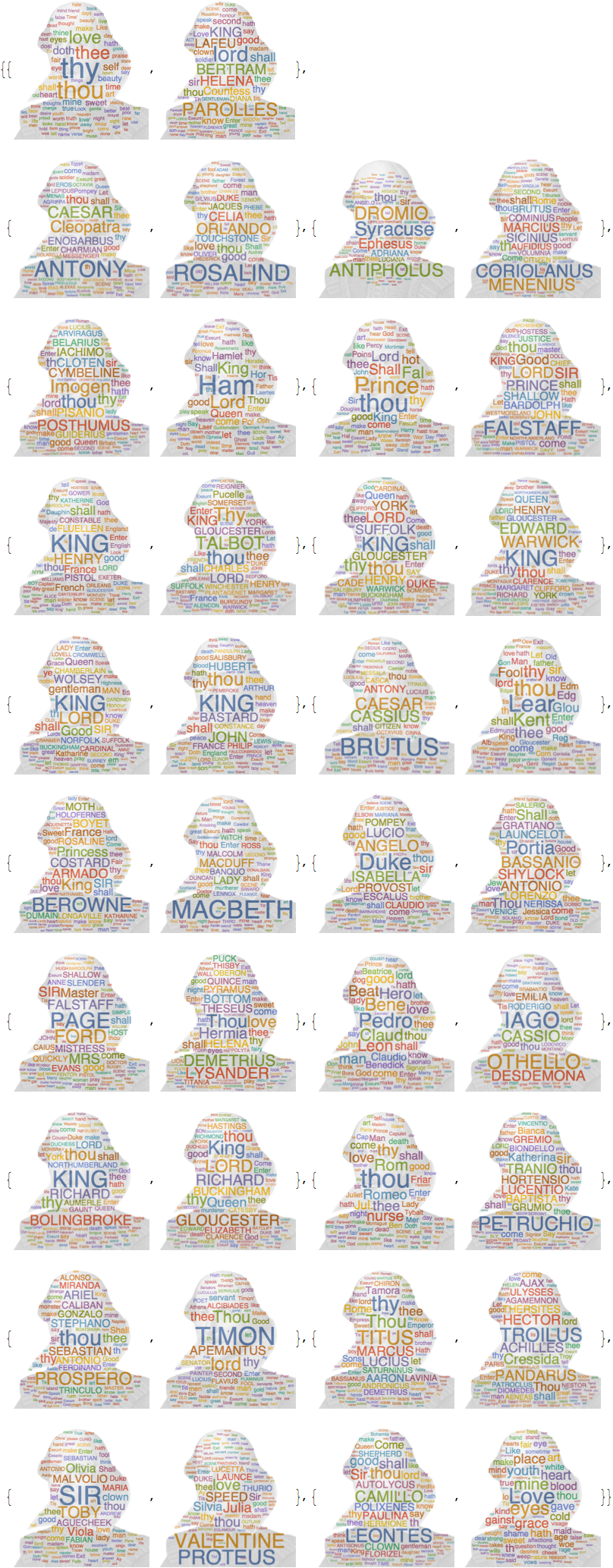
Ok. Let's do that for all texts:

Monitor[wordclouds = 
   Table[{alltexts[[k, 1]], 
     cloud = Image[WordCloud[DeleteStopwords[TextWords[alltexts[[k, 2]]]], mask, IgnoreCase -> True]]; 
     ImageCompose[cloud, {ImageResize[img, ImageDimensions[cloud]], 0.2}]}, {k, 1,Length[titles]}];, k]

and plot it:

ArrayReshape[wordclouds[[All, 2]], {19, 2}] // TableForm

enter image description here

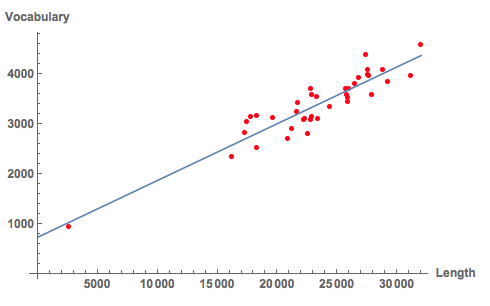
We can now also count the words per text and see how many different words Shakespeare uses:

textlength = Transpose[{alltexts[[All, 1]], Length[TextWords[#]] & /@ alltexts[[All, 2]]}];
textvocabulary = Transpose[{alltexts[[All, 1]], Length[DeleteDuplicates[ToLowerCase[DeleteStopwords[TextWords[#]]]]] & /@ alltexts[[All, 2]]}];

Here is a representation of that:

Show[
ListPlot[Table[Tooltip[{textlength[[k, 2]], textvocabulary[[k, 2]]}, textlength[[k, 1]]], {k, 1, Length[textlength]}], 
PlotStyle -> Directive[Red], AxesLabel -> {"Length", "Vocabulary"}, LabelStyle -> Directive[Bold, Medium]], 
Plot[Evaluate@Normal[LinearModelFit[Transpose[{textlength[[All, 1]], textlength[[All, 2]], textvocabulary[[All, 2]]}][[All, {2, 3}]], x, x]], {x, 0,32000}]]

enter image description here

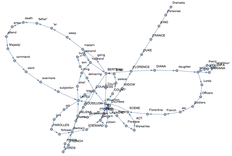
We can also construct something which is like a semantic network. Basically, we delete all Stopwords and build a network of the sequences of remaining words:

Graph[Rule @@@ Partition[DeleteStopwords[TextWords[alltexts[[2, 2]]]], 2, 1][[1 ;; 100]], VertexLabels -> "Name"]

enter image description here

If we want to be really fancy about it, we can do the whole thing in 3D:

Graph3D[Rule @@@ Partition[DeleteStopwords[TextWords[alltexts[[2, 2]]]], 2, 1][[1 ;; 100]], ImageSize -> Large, VertexLabels -> "Name", VertexLabelStyle -> Directive[Red, Italic, 10]]

enter image description here

Well, that's not a lot, but perhaps a starting point.

Cheers,

M.

POSTED BY: Marco Thiel
Reply to this discussion
Community posts can be styled and formatted using the Markdown syntax.
Reply Preview
Attachments
Remove
or Discard

Group Abstract Group Abstract