Group Abstract Group Abstract

Message Boards Message Boards

400th anniversary of Shakespeare's death

Posted 11 years ago

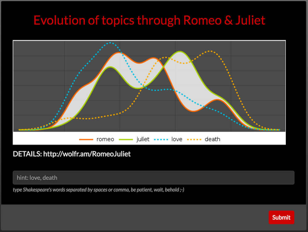
NOTE: the actual APP that does some analysis of Shakespeare's "Romeo and Juliet" is located HERE. Please wait through a potential little load or evaluation times, it is computing ! ;-) Read below and through comments for many ideas on Shakespeare's data mining.
enter image description here

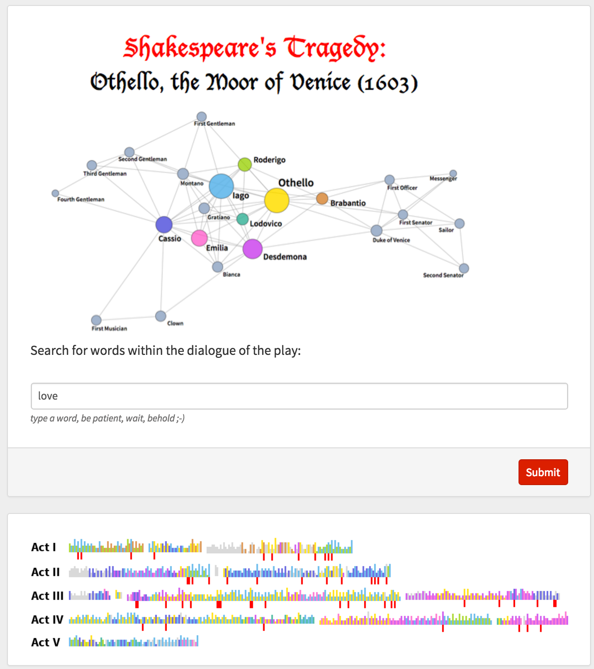
I also highly recommend reading recent related blog by Jofre Espigule and checking out his Wolfram Cloud app that does some social and linguistic visualizations of the Shakespeare's texts:
enter image description here

April 23, 2016 marks 400th anniversary of Shakespeare’s death. Just a few decades of life's work produced texts that fascinate humanity for already 400 years. This centuries-old fascination tells us Shakespeare's works highlight the perpetual social and cultural phenomena. And also that Shakespeare is a seldom genius, a true master of the written and spoken word. But have you ever thought that Shakespeare's texts can be deemed as data? Perhaps Emerging filed of digital humanities can tell us what to read between the lines. Modern technologies can provide a new insight into social networks of characters, semantic, statistical and other properties of corpus that is usually considered of only high artistic value. Is there a pattern in the art?

Could you think of data mining analysis or visualizations to apply to Shakespeare's works? Please share your thoughts! Dive with Wolfram technologies into infinite depths of Shakespeare's data.

EXAMPLE: Storyline

Imagine I would like to see in a few quick pictures how the dramatic development of events propagates through a play. I consider "Romeo and Juliet" and download full text as a string (lower-casing all words):

romeojuliet = ToLowerCase[Import["http://shakespeare.mit.edu/romeo_juliet/full.html"]];

Now I will write a function drama that displays the density of a specific word in a play. It is done by indexing positions of words in the text and then running SmoothKernelDistribution algorithm hidden inside SmoothHistogram function that also plots the density:

drama[keywords_List] := With[
  {pos = StringPosition[romeojuliet, #][[All, 1]] & /@ keywords},
  SmoothHistogram[pos,
   Frame -> None, BaseStyle -> White,
   PlotLegends -> Placed[keywords, {{.93, .8}}],
   AspectRatio -> 1/3, ImageSize -> 700, PlotTheme -> "Marketing",
   PlotStyle -> {Automatic, Automatic, Dashed, Dashed, Dashed},
   Filling -> {1 -> {2}}, FillingStyle -> Directive[White, Opacity[.8]]]]

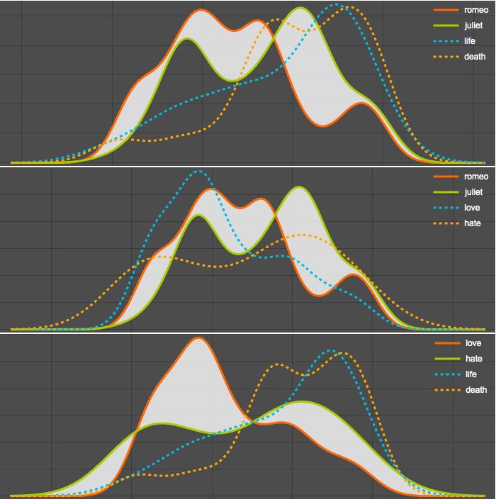
And now with a few computations drama reads the play and announces the verdict with just 3 images. Visually we see clearly what was important as the time went by. The 3rd image of interplay between "love", "hate", "life", and "death" speaks the most.

drama[{"romeo", "juliet", "life", "death"}]
drama[{"romeo", "juliet", "love", "hate"}]
drama[{"love", "hate", "life", "death"}]
enter image description here

To make a cloud app, we need to modify function a bit and use CloudDeploy.

dramaFORM[keywords_String] := Rasterize@Module[
   {pos, leg, keys = TextWords[ToLowerCase[keywords]]},
   leg = {"romeo", "juliet"}~Join~keys;
   pos = StringPosition[romeojuliet, #][[All, 1]] & /@ leg;
   SmoothHistogram[DeleteCases[pos, {} | {_Integer}],
    Frame -> None, PlotLegends -> Placed[leg, Bottom],
    AspectRatio -> 1/3, ImageSize -> 700, PlotTheme -> "Marketing",
    PlotStyle -> {Automatic, Automatic}~Join~Table[Dashed, {Length[leg] - 2}],
    Filling -> {1 -> {2}}, FillingStyle -> Directive[White, Opacity[.8]]]]

CloudDeploy[FormFunction[{
    "x" -> <|"Label" -> "", 
    "Interpreter"->"String",
    "Hint"->"hint: love, death",
    "Help"->Style["type Shakespeare's words separated by spaces or comma, be patient, wait, behold ;-)",Italic]|>}, 
    dramaFORM[#x]&,
    AppearanceRules-><|
    "Title" -> Grid[{{"Evolution of topics through Romeo & Juliet"},{Spacer[{10,5}]},{img}},Alignment->Center], 
    "Description" -> "DETAILS:  http://wolfr.am/RomeoJuliet "|>,
    FormTheme -> "Black"],
"RomeoAndJuliet",   
Permissions->"Public"]

EXAMPLE: Wordcloud

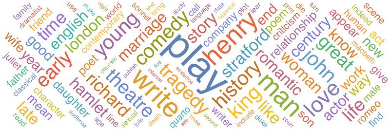
It is also interesting to know how modern society sees Shakespeare. The code below for the word cloud runs over Encyclopedia Britannica article about Shakespeare.

text=Import["http://www.britannica.com/print/article/537853"];
base[w_]:=With[{tmp=WordData[w,"BaseForm","List"]}, If[(Head[tmp]===Missing)||tmp==={},w,tmp[[1]]]];
SetAttributes[base,Listable];
tst=Quiet[base[TextWords[StringDelete[DeleteStopwords[ToLowerCase[text]],DigitCharacter..]]]];
blackLIST={"shakespeare","william","th","iii","iv","vi"};
WordCloud[DeleteCases[DeleteCases[tst,_First],Alternatives@@blackLIST],
    WordOrientation->{{-\[Pi]/4,\[Pi]/4}},AspectRatio->1/3,
    ScalingFunctions->(#^.01&),ImageSize->800]
enter image description here

DATA & CODE SOURCES:

POSTED BY: Vitaliy Kaurov
8 Replies

Here is my little contribution which is based on Chris Wilson's Wolfram Summer School side project about "Book Colors".

  • Gather a list of Color Names:

    colornames = {" alice blue ", " antique white ", " aqua ", " aquamarine ", " azure ", " beige ", " bisque ", " black ", " blanched almond ", " blue ", " blue violet ", " brown ", " burly wood ", " cadet blue ", " chartreuse ", " chocolate ", " coral ", " cornflower blue ", " cornsilk ", " crimson ", " cyan ", " dark blue ", " dark cyan ", " dark golden rod ", " dark gray ", " dark green ", " dark khaki ", " dark magenta ", " dark olive green ", " dark orange ", " dark orchid ", " dark red ", " dark salmon ", " dark sea green ", " dark slate blue ", " dark slate gray ", " dark turquoise ", " dark violet ", " deep pink ", " deep sky blue ", " dim gray ", " dodger blue ", " fire brick ", " floral white ", " forest green ", " fuchsia ", " gainsboro ", " ghost white ", " gold ", " golden rod ", " gray ", " green ", " green yellow ", " honey dew ", " hot pink ", " indian red ", " indigo ", " ivory ", " khaki ", " lavender ", " lavender blush ", " lawn green ", " lemon chiffon ", " light blue ", " light coral ", " light cyan ", " light gray ", " light green ", " light pink ", " light salmon ", " light sea green ", " light skyblue ", " light slate gray ", " light steel blue ", " light yellow ", " lime ", " lime green ", " linen ", " magenta ", " maroon ", " medium blue ", " medium orchid ", " medium purple ", " medium sea green ", " medium slate blue ", " medium spring green ", " mediumturquoise ", " medium violetred ", " midnight blue ", " mint cream ", " misty rose ", " moccasin ", " navajo white ", " navy ", " old lace ", " olive ", " olive drab ", " orange ", " orange red ", " orchid ", " pale golden rod ", " pale green ", " pale turquoise ", " pale violet red ", " papaya whip ", " peach puff ", " peru ", " pink ", " plum ", " powder blue ", " purple ", " red ", " rosy brown ", " royal blue ", " saddle brown ", " salmon ", " sandy brown ", " sea green ", " sea shell ", " sienna ", " silver ", " sky blue ", " slate blue ", " slate gray ", " snow ", " spring green ", " steel blue ", " teal ", " thistle ", " tomato ", " turquoise ", " violet ", " wheat ", " white ", " white smoke ", " yellow ", " yellow green "};
    
  • Use the color Interpreter to get them in the WL:

    colors = Interpreter["Color"][colornames]
    

colors

  • Make a PieChart of the StringCounts of these color names:

    Column@Table[
    link="http://shakespeare.mit.edu/"<>works<>"/full.html";
    text=ToLowerCase[Import[link]];
    PieChart[
    ParallelMap[StringCount[text,#]&,colornames],
    ChartStyle->colors,
    PlotLabel->Hyperlink[TextCases[text,"Line",1],link],
    LabelingFunction->"RadialCenter",
    ChartLabels->Placed[colornames,"RadialCallout"],
    ImageSize->600],
    {works,StringSplit[#,"/"][[-2]]&/@Import["http://shakespeare.mit.edu/","Hyperlinks"][[3;;-8]]}]
    

Enjoy!

Attachments:
POSTED BY: Bernat Espigulé
POSTED BY: David Gathercole

You are completely right David! Somehow I assumed that was due to the domineering qualities of red:

Red - is a bold color that commands attention! Red gives the impression of seriousness and dignity, represents heat, fire and rage, it is known to escalate the body's metabolism. Red can also signify passion and love. Red promotes excitement and action. It is a bold color that signifies danger, which is why it's used on stop signs. Using too much red should be done with caution because of its domineering qualities. Red is the most powerful of colors. The Psychology of Color

Thanks for noticing it. I've just updated the color names above:

colornames = StringJoin[" ", #, " "] & /@ colornames;

Now it looks just right:

Colors Shakespeare

POSTED BY: Bernat Espigulé
Attachments:
POSTED BY: Marco Thiel

I took this opportunity to use the Wolfram Language on XML documents, specifically a TEI (http://www.tei-c.org) version of "The Tempest," which can be found at the University of Oxford Text Archive (http://ota.ox.ac.uk).

We start by importing the xml document as an XMLObject.

tempestxml = Import["http://ota.ox.ac.uk/text/5725.xml", "XMLObject"];

After exploring the document a little, I found that I could extract lines by a specific speaker with Cases. Here is how to get all the lines spoken by Prospero:

proslines = 
  Cases[tempestxml, XMLElement["sp", {}, {XMLElement["speaker", _, {"Pros."}], line_}] :> line, Infinity];

I made a WordCloud of those lines, only to discover that we lack Elizabethan stopwords:

WordCloud[DeleteStopwords@ToLowerCase@TextWords[StringRiffle[Flatten[proslines//.XMLElement[_,_,content_]:>content]]]]

First Prospero WordCloud

It's much more satisfying after a minor tweak:

WordCloud[DeleteCases[DeleteStopwords@ToLowerCase@TextWords[StringRiffle[Flatten[
    proslines //. XMLElement[_, _, content_] :> content]]], "thee" | "thou" | "thy"]]

Second Prospero WordCloud

Why limit ourselves to one character, though?

linesbychar = First@First@# -> Last /@ # & /@ GatherBy[Cases[tempestxml, 
    XMLElement["sp", {}, {XMLElement["speaker", _, {char_}], line_}] :> char -> line, Infinity], First]; 

Grid[Partition[Column@{First@#, WordCloud[DeleteCases[DeleteStopwords@ToLowerCase@TextWords[
               StringRiffle[Flatten[Last@# //. XMLElement[_, _, content_] :> content]]], 
                    "thee" | "thou" | "thy"]]} & /@ linesbychar, 6], Frame -> All, Alignment -> Left]

WordClouds for all characters

We don't have to limit ourselves to characters, we can make WordCloud for each scene. In this document, each scene is contained in a <div>

scenes = Cases[tempestxml, XMLElement["div", _, div_] :> div, Infinity];
Grid[Partition[Column[{First@#, WordCloud[DeleteCases[DeleteStopwords@ToLowerCase@TextWords[
           StringRiffle[Flatten[Cases[Last@#, XMLElement["ab", _, line_] :> line, Infinity] //. XMLElement[_, _, content_] :> content]]],
             "thee" | "thou" | "thy"]]}] & /@ ((Replace[Flatten[Cases[#, 
                XMLElement["head", _, h_] :> (h //. XMLElement[_, _, content_] :> content)]], {s_String} :> s] -> Rest@#) & /@ scenes), 5],                 
                    Frame -> All, Alignment -> Left]

a WordCloud for each scene

POSTED BY: Aaron Enright
POSTED BY: Marco Thiel
Posted 11 years ago

@Marco Thiel , you are indeed fast. My take on the graph of characters, leaving the conversations between characters.

data = SemanticImport[
   "c:\\Users\\Diego\\Downloads\\will_play_text.csv", Automatic, 
   "Rows", Delimiters -> ";"];
data[[All, 
    4]] = (ToExpression@StringSplit[#, "."] & /@ 
     data[[All, 4]]) /. {} -> {Missing[Empty], Missing[Empty], 
     Missing[Empty]};
sentiment = 
  Classify["Sentiment", data[[All, 6]]] /. {"Neutral" -> 0, 
    "Positive" -> 1, "Negative" -> -1, Indeterminate -> 0};
data[[All, 6]] = Transpose[{data[[All, 6]], sentiment}];
ds = Dataset[
  AssociationThread[{"ID", "Play", "Phrase", "Act", "Scene", "Line", 
      "Character", "Text", "Sentiment"}/@ (Flatten /@ data)];
getEdges[play_, act_, scene_] := 
 DirectedEdge[#[[1]], #[[2]]] & /@ 
  Partition[
   ds[Select[#Play == play &] /* Union, {"Act", "Scene", "Phrase", 
       "Character"}][Select[#Act == act && #Scene == scene &], 
     "Character"] // Normal, 2, 1]
getGraph[play_] := 
 Graph[Flatten[
   getEdges[#[[1]], #[[2]], #[[3]]] & /@ (ds[
         Select[#Play == play &] /* Union, {"Play", "Act", "Scene"}] //
         Normal // Values // Most)], VertexLabels -> "Name", 
  ImageSize -> 1024]
getGraph["Othello"]

enter image description here

Well, what about how many movies or TV Shows were made of the most famous plays?

plays={"Macbeth", "Romeo and Juliet", "Othello", "Hamlet", "King Lear", \
"Richard III", "The Tempest", "Merry Wives of Windsor", "Titus \
Andronicus"}
movies[play_] := 
 Import["http://www.imdb.com/find?q=" ~~ 
    StringReplace[play, " " -> "%20"] ~~ 
    "&s=tt&exact=true&ref_=fn_tt_ex", "Data"][[4, 1]]

shakespeareMovies = {Length@movies[#], #} & /@ plays // Sort // 
   Transpose;
BarChart[#[[1]], BarOrigin -> Left, ChartLabels -> #[[2]], 
   Frame -> True, 
   PlotLabel -> "Shakespeare Based Movies"] &@shakespeareMovies

BarChart[#[[1]], BarOrigin -> Left, ChartLabels -> #[[2]], 
   Frame -> True, PlotLabel -> "Shakespeare Based Movies", 
   PlotTheme -> "Detailed", ImageSize -> Large] &@shakespeareMovies

enter image description here

POSTED BY: Diego Zviovich
POSTED BY: Marco Thiel
Reply to this discussion
Community posts can be styled and formatted using the Markdown syntax.
Reply Preview
Attachments
Remove
or Discard