Message Boards Message Boards

Dancing with friends and enemies: boids' swarm intelligence

Posted 12 years ago
The latest way I have found to use my expensive math software for frivolous entertainment is this. Here's is a way to describe it.
  • 1000 dancers assume random positions on the dance-floor.
  • Each randomly chooses one "friend" and one "enemy".
  • At each step every dancer
    • moves 0.5% closer to the centre of the floor
    • then takes a large step towards their friend
    • and a small step away from their enemy.
  • At random intervals one dancer re-chooses their friend and enemy

Randomness is deliberately injected. Here is the dance...
n = 1000;
r := RandomInteger[{1, n}];
f := (#/(.01 + Sqrt[#.#])) & /@ (x[[#]] - x) &;
s := With[{r1 = r}, p[[r1]] = r; q[[r1]] = r];
x = RandomReal[{-1, 1}, {n, 2}];
{p, q} = RandomInteger[{1, n}, {2, n}];
Graphics[{PointSize[0.007], Dynamic[If[r < 100, s];
Point[x = 0.995 x + 0.02 f[p] - 0.01 f[q]]]}, PlotRange -> 2]


Thanks to Vitaliy for posting this on my behalf, complete with animations :-)

Background: I had read somewhere that macro-scale behaviour of animal swarms (think of flocks of starlings or shoals of herring) is explained by each individual following very simple rules local to their vicinity, essentially 1) try to keep up and 2) try not to collide. I started trying to play with this idea in Mathematica, but it was rather slow to identify the nearest neighbours of each particle. So I wondered what would happen if each particle acted according to the locations of two other particles, regardless of their proximity. The rule was simply to move away from one and towards the other.

The contraction (x = 0.995 x) was added to prevent the particle cloud from dispersing towards infinity or drifting away from the origin. I tweaked the "towards" and "away" step sizes to strike a balance between the tendency to clump together and to spread apart (if you make the step sizes equal you get something more like a swarm of flies). With each particle's attractor and repeller fixed, the system finds a sort of dynamic equilibrium, so to keep things changing I added a rule to periodically change the attractor and repeller for one of the particles. The final adjustment was to make the "force" drop towards zero for particles at very close range. This helps to stop the formation of very tight clumps, and also prevents a division-by-zero error when a particle chooses itself as its attractor or repeller.

The description of the system as a dance was an attempt to explain the swirling pattern on the screen without using mathematical language. I'd love to see what other "dances" can be created with other simple rules.
POSTED BY: Simon Woods
29 Replies
Posted 12 years ago
What you call "frivolous entertainment," social scientists (including socio-physicists) call 'serious research.' I prefer your description, but then IMO, most social science simulations, if viewed as research (which they do), should be identified as ridiculous pseudo-science.
POSTED BY: Richard Gaylord
@Jari Kirma:  Great, Thanks a lot
POSTED BY: Mohamed Zaghloul
Posted 12 years ago
 @MohamedZaghloul: you can export per-frame data in the following way, in this case 100 frames:
n = 1000;
r := RandomInteger[{1, n}];
f := (#/(.01 + Sqrt[#.#])) & /@ (x[[#]] - x) &;
s := With[{r1 = r}, p[[r1]] = r; q[[r1]] = r];
x = RandomReal[{-1, 1}, {n, 2}];
{p, q} = RandomInteger[{1, n}, {2, n}];

Scan[If[r < 100, s]; Export["swarm_" <> ToString@# <> ".dat", x = 0.995 x + 0.02 f[p] - 0.01 f[q]] &, Range[100]]
This produces files swarm_1.dat, swarm_2.dat, ... swarm_100.dat.

Format of export is decided by file extension (".dat" in this case for Table format), or third parameter to Export (see documentation).

You can also "play back" such a sequence of files, albeit it may be a bit slow this way:
i = 1;
p = {};
Graphics[{PointSize[0.007],
  Dynamic[With[{f = "swarm_" <> ToString@i <> ".dat"},
    If[FileExistsQ[f], i++; p = Point[Import[f]], p]]]},
  PlotRange -> 2]
POSTED BY: Jari Kirma
Woah!!!
POSTED BY: Safi Ahmed
Improved Manipulate, 2D/3D Tab, Color Styles, Equation Labels ... Enjoy!
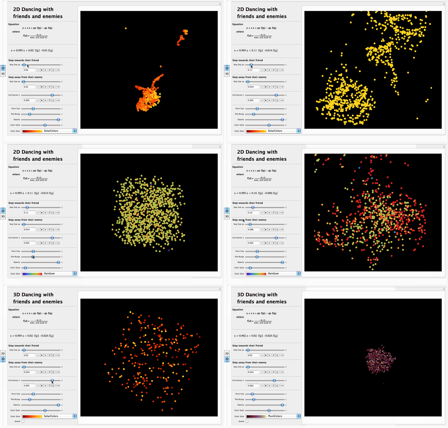


 TabView[{
   "2D" -> Manipulate[n = 1000;
     r := RandomInteger[{1, n}];
     f := (#/(.01 + Sqrt[#.#])) & /@ (x[[#]] - x) &;
     s := With[{r1 = r}, p[[r1]] = r; q[[r1]] = r];
     x = RandomReal[{-1, 1}, {n, 2}];
     {p, q} = RandomInteger[{1, n}, {2, n}];
     Graphics[{Opacity[opacity], PointSize[size],
       Dynamic[If[r < 200, s];
       Point[y = x; x = c*x + ps*f[p] - qs*f[q],
        VertexColors -> (ColorData[col][color*Norm[#]] & /@ (x - y))]]}, PlotRange -> Range, ImageSize -> {700, 600},
     Background -> Black], Delimiter, Style["   2D Dancing with
        friends and enemies", Bold, Large], Delimiter, Style["Equation
                       x = c x + ps f[p] - qs f[q]
          where
       \!\(\*FormBox[\(\(\\\ \\\ \\\ \\\ \\\ \\\ \\\ \\\ \\\ \\\ \\\ \
\\\ \\\ \\\ \\\ \\\ \\\ \\\ \\\ \\\ \\\ \\\ \\\ \\\ \\\ \\\ \\\ \\\ \
\\\ \)\(f[a] = \*FractionBox[\((a - x)\), \(0.01 + \*SqrtBox[\(\((a - \
x)\) . \((a - x)\)\)]\)]\)\),
     TraditionalForm]\)
       ", Bold, Medium], Delimiter,
    Dynamic[Graphics[{Style[
        Text@TraditionalForm@
          Style[Row[{"x = ", c "x + ", ps " f[p] -", qs "f[q]"}]],
        15]}, ImageSize -> {240, 50}]], Delimiter,
    Style["Step towards their friend", Bold,
     Medium], {{ps, 0.02, "Step Size ps"}, 0, 1,Appearance -> "Open"}, Delimiter,
    Style["Step away from their enemy", Bold,
     Medium], {{qs, 0.01, "Step Size qs"}, 0, 1, Appearance -> "Open"},
    Delimiter, {{c, 0.995, "Contraction c"}, 0.5, 1.1,  Appearance -> "Open"},
    Delimiter, {{size, 0.015, "Point Size"}, 0.001, 0.05}, {{Range, 1, "Plot Range"}, 0.1, 5}, {{opacity, 1, "Opacity"}, 0.1, 1}, {{color, 62, "Color Scale"}, 0, 100},
    Control[{{col, "SolarColors", "Color Style"},
      (# -> Row[{Show[ColorData[#, "Image"], ImageSize -> 100], Spacer[10], #}]) & /@ ColorData["Gradients"], PopupMenu}],
     ControlPlacement -> Left],
 
  "3D" -> Manipulate[n = 1000;
    r := RandomInteger[{1, n}];
    f3d := (#/(.01 + Sqrt[#.#])) & /@ (x3d[[#]] - x3d) &;
    s := With[{r1 = r}, p[[r1]] = r; q[[r1]] = r];
    x3d = RandomReal[{-1, 1}, {n, 3}];
    {p, q} = RandomInteger[{1, n}, {2, n}];
    Graphics3D[{Opacity[opacity], PointSize[size],
      Dynamic[If[r < 200, s];
       Point[y = x3d; x3d = c*x3d + ps*f3d[p] - qs*f3d[q],
        VertexColors -> (ColorData[col][color*Norm[#]] & /@ (x3d - y))]]}, PlotRange -> Range, ImageSize -> {700, 600},
     Background -> Black, Boxed -> boxed], Delimiter,
    Style["   3D Dancing with
        friends and enemies", Bold, Large], Delimiter, Style["Equation
                       x = c x + ps f[p] - qs f[q]
          where
       \!\(\*FormBox[\(\(\\\ \\\ \\\ \\\ \\\ \\\ \\\ \\\ \\\ \\\ \\\ \
\\\ \\\ \\\ \\\ \\\ \\\ \\\ \\\ \\\ \\\ \\\ \\\ \\\ \\\ \\\ \\\ \\\ \
\\\ \)\(f[a] = \*FractionBox[\((a - x)\), \(0.01 + \*SqrtBox[\(\((a - \
x)\) . \((a - x)\)\)]\)]\)\),
     TraditionalForm]\)
       ", Bold, Medium], Delimiter,
    Dynamic[Graphics[{Style[
        Text@TraditionalForm@
          Style[Row[{"x = ", c "x + ", ps " f[p] -", qs "f[q]"}]],
        15]}, ImageSize -> {240, 50}]], Delimiter,
    Style["Step towards their friend", Bold,
     Medium], {{ps, 0.02, "Step Size ps"}, 0, 1, Appearance -> "Open"}, Delimiter,
    Style["Step away from their enemy", Bold,
     Medium], {{qs, 0.01, "Step Size qs"}, 0, 1, Appearance -> "Open"},
    Delimiter, {{c, 0.995, "Contraction c"}, 0.5, 1.1, Appearance -> "Open"},
    Delimiter, {{size, 0.015, "Point Size"}, 0.001, 0.05}, {{Range, 1, "Plot Range"}, 0.1, 5}, {{opacity, 1, "Opacity"}, 0.1, 1}, {{color, 62, "Color Scale"}, 0, 100},
    Control[{{col, "SolarColors", "Color Style"},
      (# ->Row[{Show[ColorData[#, "Image"], ImageSize -> 100],  Spacer[10], #}]) & /@ ColorData["Gradients"],
      PopupMenu}], {boxed, {True, False}}, ControlPlacement -> Left]},
  ControlPlacement -> Left]
Thanks to Andre and Vitaliy for suggesting some of these improvements.
POSTED BY: Bernat Espigulé
Posted 12 years ago
Here is a variant of this with explicitly chained friendly rings (in this case two). Enemies are still random, but not modified after creation:
n = 2000;
f := (#/(.01 + Sqrt[#.#])) & /@ (x[[#]] - x) &;
x = Table[{Sin[a], -Cos[a]}, {a, 0., 2 \[Pi], 2 \[Pi]/(n - 1)}];
p = Table[Mod[i + 1, n] + 1, {i, n}];
q = RandomInteger[{1, n}, n];
Graphics[{PointSize[0.007], Dynamic[
   Point[x = 0.995 x + 0.02 f[p] - 0.01 f[q]]]}, PlotRange -> 2]

Amount of rings involved can be modified by adding something else than 1 to i inside Mod. 0 gives single ring, 2 three, and so on (as far as n is multiple of amount of rings).
POSTED BY: Jari Kirma
Simon,
Animal swarm: it could be you saw the original flock study which was done by my friend Craig Reynolds: http://www.red3d.com/cwr/boids/ and published in SIGGRAPH 1987...

POSTED BY: Luc Barthelet
This post was discussed on Reddit which resulted in recreation of the algorithm in programming language called Processing using 1,000,000 particles and simulation running over night! Here is the link to the VIDEO:

POSTED BY: Vitaliy Kaurov
@Vitaliy, looks like Community is getting popular. I also did an overnight simulation the day this discussion was started. This is the compressed ouput of the original (53MB ) 200,000 particles simulation with Mathematica:


The arrow of time has been reversed in this GIF. It's like traveling back to the Big Bang!
POSTED BY: Bernat Espigulé
Posted 10 months ago

Hi Vitaliy,

Thank you for the nice post.

Is there any application of this issue in environmental or civil engineering?

Thank you for your time.

Cheers,

POSTED BY: Alex Teymouri
... and this is the code for generating animated GIFs using Spheres instead of Points:
 n = 1000;
 r := RandomInteger[{1, n}];
 f := (#/(.01 + Sqrt[#.#])) & /@ (x[[#]] - x) &;
 s := With[{r1 = r}, p[[r1]] = r; q[[r1]] = r];
 x = RandomReal[{-1, 1}, {n, 3}];
 {p, q} = RandomInteger[{1, n}, {2, n}];
 Export["Dancing_Spheres.gif",
  Table[
 Graphics3D[
Rotate[{Yellow, Dynamic[If[r < 100, s]; Sphere[x = 0.995 x + 0.02 f[p] - 0.01 f[q], 0.04]]}, th, {0, 0, 1}],
ImageSize -> {700, 500}, Background -> Black, Boxed -> False, PlotRange -> 2],
{th, 0, 2 Pi, 0.03}]]


For two-dimensional animations, one can use the method explained in my discussion Visualizing Animated GIFs Along The Time Dimension With Image3D to keep track of the swarm's complex dynamics.

 ? ? Time
POSTED BY: Bernat Espigulé
Amazing! Here is my Manipulate to add extra excitement to this swarm dance.
 n = 1000;
 r := RandomInteger[{1, n}];
 f := (#/(.01 + Sqrt[#.#])) & /@ (x[[#]] - x) &;
 s := With[{r1 = r}, p[[r1]] = r; q[[r1]] = r];
 x = RandomReal[{-1, 1}, {n, 3}];
 {p, q} = RandomInteger[{1, n}, {2, n}];
 Manipulate[
  Graphics3D[
   Rotate[
   {White, PointSize[0.002], Dynamic[If[r < 200, s];
     Point[y = x; x = 0.995*x + ps*f[p] - qs*f[q],
      VertexColors -> (ColorData["TemperatureMap"][
           Color*Norm[#]] & /@ (x - y))]]},
   Rotate3D, {0, 0, 1}], PlotRange -> Range, ImageSize -> {700, 500},
  Background -> Black, Boxed -> False],
{Rotate3D, 0, 2 Pi},
{{Range, 2}, 0.1, 5},
{{Color, 62}, 0, 100},
Delimiter, Style["Step towards their friend", Bold, Medium],
{{ps, 0.02}, 0, 1},
Delimiter, Style["Step away from their enemy", Bold, Medium],
{{qs, 0.01}, 0, 1}, ControlPlacement -> Left]
POSTED BY: Bernat Espigulé
I actually like what Bernat did very much. It gave me an opportunity to find an interesting range of parameters where almost perfect multiple interacting ring systems can form { Step towards friend = 0.068, Step away from enemy = 0.006 }. This is pretty mesmerizing to watch:

POSTED BY: Vitaliy Kaurov
@Vitaliy, your example is the best illustration of blowing smoke ring ever.
POSTED BY: Shenghui Yang
Thanks Vitaliy. Good catch! I got some tubular structures in-between yours and Woods' parameters range. Tip, the Color slider can be always adjusted to obtain a nice chromatic palette.

POSTED BY: Bernat Espigulé
Simon, if you want to deal with physical neighbors you can get quite reasonable speed using a NearestFunction, created once per time step. An alternative might be to keep track of which particle is in what grid sector, but the extra coding effort could take you from frivolous entertainment to the seriously demented hobbies level.
POSTED BY: Daniel Lichtblau
Posted 12 years ago
Daniel, LOL, yes it's a fine line! My rule of thumb is that when you start needing version control you're not having fun any more :-)
POSTED BY: Simon Woods
Here is some test with colors based on velocity using 3D code.
 n=3000;
 r:=RandomInteger[{1,n}];
 f:=(#/(.01+Sqrt[#.#]))&/@(x[[#]]-x)&;
 s:=With[{r1=r},p[[r1]]=r;q[[r1]]=r];
 x=RandomReal[{-1,1},{n,3}];
 {p,q}=RandomInteger[{1,n},{2,n}];
 Graphics3D[{
     White,
     PointSize[0.002]
    ,Dynamic[
        If[r<200,s];
        Point[y=x;x=0.995x+0.02f[p]-0.01f[q],VertexColors->(ColorData["TemperatureMap"][50Norm[#]]&/@(x-y))]
    ]
    },PlotRange->2,Background->Black]

POSTED BY: Rodrigo Murta
Here is a video which shows a longer sequence than the animated gif above:

WATCH VIDEO
POSTED BY: Arnoud Buzing
NetLogo is very suitable for writing these kinds of simulations.  It also has a Mathematica interface which makes it possible to drive the simulations from Mathematica and send back measurements to it.
POSTED BY: Szabolcs Horvát
Posted 12 years ago
Throwing out some probably obvious observations:

The driving forces in the 'dancing clouds' seem to be buddy cliques, where all members of such a subset of dancers are friends with one another; the 'cloud tails' are chains of followers where one wants to be friends with the previous one in the chain, and the first wants to be friends with somebody in one of the buddy cliques.
One should be able to show this quickly with a directed friendship graph like Graph[Table[DirectedEdge[r, p[[ r ]]], {r, 1000}].

The repulsion from enemies prevents condensation into a single point, and the 'changes of mind' create the ever-changing dynamics.

However to make it a choreographed dance I would assume one would need to fix the relationship structure and place the dancers in a nice pattern, initially. I wonder there how stable such dance patterns would be, as a function of the step sizes towards friends and away from enemies, whether the forming patterns would be unique, given an underlying relationship structure, and whether one could choreograph transitions between individual dance patterns, by individual step disturbances or friendship structure disturbances.

But maybe I'm just taking this too far instead of just enjoying these wonderful random dances.

Thank you, Simon!
POSTED BY: Peter Fleck
I cannot call this perfect without some visual techno ;-) visualize the distance between the some pair of data points, scaled to 1/3 of the actual length; the bigger the circle, the farther they are apart
 n = 1000;
 r := RandomInteger[{1, n}];
 f := (#/(.01 + Sqrt[#.#])) & /@ (x[[#]] - x) &;
 s := With[{r1 = r}, p[[r1]] = r; q[[r1]] = r];
 x = RandomReal[{-1, 1}, {n, 2}];
 {p, q} = RandomInteger[{1, n}, {2, n}];
 Dynamic[
  If[r < 100, s];
  x = 0.995 x + 0.02 f[p] - 0.01 f[q];
Graphics[Flatten[
   Table[{ColorData["Rainbow"][Norm[x[[i]] - x[[j]]]/3],
     Disk[{i, j}, Norm[x[[i]] - x[[j]]]/3]}, {i, 1, 10}, {j, i + 1,
     11}]
   , 1], PlotRange -> {{-1, 12}, {-1, 12}}]
]

POSTED BY: Shenghui Yang
This is so nice yet the code is extremely concise!
POSTED BY: Shenghui Yang
Very cool. For 3D just do:
x = RandomReal[{-1, 1}, {n, 2}];
(*for*)
x = RandomReal[{-1, 1}, {n, 3}];
And Graphics to Graphics3D.
The velocity worked just nice.
POSTED BY: Rodrigo Murta
Rodrigo, - nice observation! One can also rotate 3D graphics without interference with simulation. I added points up to 2000 and also added SphericalRegion -> True for nice rotation action. This simulation produces nice spiral rotational motions, like galaxy or tornado or vortex formation. I wonder why that is.
 n = 2000;
 r := RandomInteger[{1, n}];
 f := (#/(.01 + Sqrt[#.#])) & /@ (x[[#]] - x) &;
 s := With[{r1 = r}, p[[r1]] = r; q[[r1]] = r];
 x = RandomReal[{-1, 1}, {n, 3}];
 {p, q} = RandomInteger[{1, n}, {2, n}];
 Graphics3D[{PointSize[0.007],
   Dynamic[If[r < 100, s];
   Point[x = 0.995 x + 0.02 f[p] - 0.01 f[q]]]}, PlotRange -> 2, SphericalRegion -> True]

POSTED BY: Vitaliy Kaurov
Hi, i have a question concerning this intersting model-----How can i export these data as a series of TXT files of these point data per frame step!!
POSTED BY: Mohamed Zaghloul
Posted 11 years ago

I am fascinated by this system , especially this simple visualization. But I still do not understand , how is that possible ? Is it the symbolism ? Or how can this be so well calculated and displayed.

POSTED BY: Max Rasumak
That's tremendous!  Particle systems are always a lot of fun.
Very nice. I wish my frivolous entertainment were that exciting.
POSTED BY: Daniel Lichtblau
Reply to this discussion
Community posts can be styled and formatted using the Markdown syntax.
Reply Preview
Attachments
Remove
or Discard

Group Abstract Group Abstract