Dear all, inspired by another great post of @Anton Antonov and in particular there by a remark of @Vitaliy Kaurov pointing to the art of knitting images I could not resist trying with Mathematica. Clearly - this problem is crying out loudly for Radon transform!

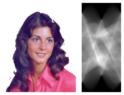
I start by choosing some example image, convert it to inverse grayscale and perform the Radon transform.
ClearAll["Global`*"]
img0 = RemoveBackground[
   ImageTrim[
    ExampleData[{"TestImage", "Girl3"}], {{80, 30}, {250, 240}}], {"Background", {"Uniform", .29}}];
img1 = ImageAdjust[ColorNegate@ColorConvert[RemoveAlphaChannel[img0], "Grayscale"]];
{xDim, yDim} = {180, 400}; (* i.e. angles between 1\[Degree] and 180\[Degree] *)

rd0 = Radon[img1, {xDim, yDim}];
ImageCollage[{img0, ImageAdjust@rd0}, Method -> "Rows",
 Background -> None, ImagePadding -> 10]

Every column of the Radon image represents a different angle of projection. So next I separate these columns into (here 180) single Radon images and do an inverse Radon transform on each:
maskLine[a_] := Table[If[a == n, 1, 0], {n, 1, xDim}];
maskImg = Table[Image[ConstantArray[maskLine[c], yDim]], {c, 1, xDim}];
rdImgs = rd0 maskImg;
ProgressIndicator[Dynamic[n], {1, xDim}]
invRadImgs =
  Table[{ImageApply[If[# > 0, #, 0] &,
     InverseRadon[rdImgs[[n]]]], -(n - 91) \[Degree]}, {n, 1, xDim}];
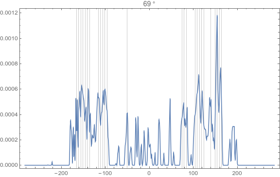
These data already represent the angle dependent intensities for backpropagation. Now one just has somehow to translate these intensities into discretely spaced lines (because this is the actual task in analogy to the above mentioned knitting ). Here is my simple attempt, which e.g. for 69° gives the following result (I am not really happy with this - there is definitely room for improvement!):

valsAngle[invRads_] := Module[{img, angle, data, l2},
   angle = Last@invRads;
   data = Max /@ (Transpose@*ImageData@*ImageRotate @@ invRads);
   l2 = Round[Length[data]/2];
   data = MapIndexed[{First[#2] - l2, #1} &, data];
   {Select[
     Times @@@ ({#1,
          If[#2 > .0003, 1, 0]} & @@@ ((Mean /@ # &)@*Transpose /@
          Partition[data, 5])), # != 0 &], angle}  (*
   limiting value of 0.0003 is just empirical! *)
   ];

va = valsAngle /@ invRadImgs;
graphicsData[va_] := Module[{u, angle},
   {u, angle} = va;
   InfiniteLine[# {Cos[angle], -Sin[angle]}, {Sin[angle],
       Cos[angle]}] & /@ u];

gd = graphicsData /@ va;
Graphics[{Thickness[.0003], gd}, ImageSize -> 600,
 PlotRange -> {{-170, 170}, {-220, 220}}]
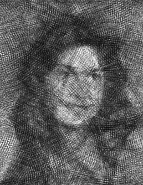
... and the result is a bunch of lines:

 Attachments: