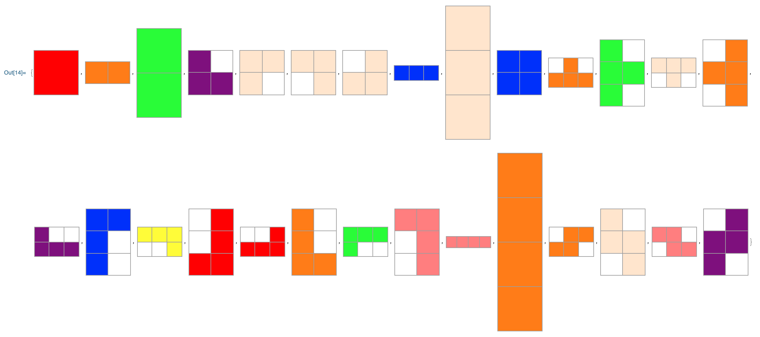
Yes, Caveat Emptor! Because we generated so much content more than was really necessary to get the point across, now we're adding more off our list of omissions with insightful results about the Project L Board Game. There's nothing better than getting carried away generating tangentially related exciting content; the purpose of Project L Board Analysis is to provide reproducibility so that we as your summer school students can verify our results and raise an open-ended, evolving solution with Q & A; there's a chance for innovation and originality, like The Story of Spikey. From a mathematical viewpoint the board game "Project L" simply asks players to solve exact cover problems given limited resources and time constraints. The description helps tremendously; Project L is the kind of thing you wanna play with your friends and learn more about because there are so many shapes like the yellow monominoes, green dominoes, orange or blue trominos, and five singly-colored tetrominos. These are called Polyominoes and there are 90 in the picture. Project L Board Analysis can be rephrased as a combinatorial problem within which the full set of tiles is the starting point, that players would build up by the end of the game. For each puzzle, the weight metrics are:
- The number of points in the top left corner,
- The grid size (or weight) of the polyomino rewards piece,
- The grid size of the to-fill-in recessed, white, inner regions.
Since the player with the highest score wins, we can assume that every point value P is in fact an expected time T = P to completion. This assumption is the number of points which is awarded in the top left corner, assuming a linear relationship between complexity and time to completion. W/T' = (T/T') * W/T. With the link between P = T, we can write W/T' = (P/T') * W/P. The player can choose three consecutive actions:
- A puzzle is drawn from the bank at no cost.
- A tile of weight N is played into the puzzle.
- A tile of weight 1 is drawn from the bank.
- A tile of weight N is traded to the bank for another of max weight N+1.
- Multiple tiles of total weight X can be played into consecutive puzzles. (This play of X per one time interval is usually the player's maximum power action, since total weight is a summation of up to four individual tile weights (players can have at max four puzzles on board). The expected time is mostly less than or equal to the actual time to completion T', based on the data science that's how most puzzles in the game are balanced.
With Harshal Gajjar's commendable method from the Tiling of Polyominoes and Brad, (thank you so much for writing it is so good that these results are effectively reproducible. Learning more about gTest and mTest is my thing.), let's take a closer look.
mirrorv[tile_] := Module[{line = {}, tMirror = {}},
  tMirror = {};
  For[i = 1, i <= Length[tile], i++,
   line = {};
   For[j = Length[tile[[1]]], j >= 1, j--,
    AppendTo[line, tile[[i, j]]];
    ];
   AppendTo[tMirror, line];
   ];
  tMirror
  ]
rotatec[tile_] := Module[{line = {}, tMirror = {}},
  tMirror = {};
  For[i = 1, i <= Length[tile[[1]]], i++,
   line = {};
   For[j = Length[tile], j >= 1, j--,
    AppendTo[line, tile[[j, i]]];
    ];
   AppendTo[tMirror, line];
   ];
  tMirror
  ]
allTiles[tile_] := Module[{list = {}},
  list = Join[NestList[rotatec, tile, 3],
    NestList[rotatec, mirrorv[tile], 3]];
  list = DeleteDuplicates[list];
  list
  ]
tiles = {
  {{1}},
  {{1, 1}},
  {{1, 0},
   {1, 1}},
  {{1, 1, 1}},
  {{1, 1},
   {1, 1}},
  {{0, 1, 0},
   {1, 1, 1}},
  {{1, 0, 0},
   {1, 1, 1}},
  {{1, 1, 1, 1}},
  {{0, 1, 1},
   {1, 1, 0}}
  }
tiles = Flatten[allTiles /@ tiles, 1];
ArrayPlot[#, ImageSize -> 100, Frame -> None, Mesh -> True,
   ColorRules -> {0 -> Transparent,
     1 ->
      Table[
       Part[{Red, Yellow, Green, Purple, Orange, LightBlue, Blue,
         Pink, LightOrange}, RandomInteger[8] + 1], 9]}] & /@ tiles
PolyominoGraph[arrayMesh_] :=
 Construct[
  With[{edges =
      ReplaceAll[MeshPrimitives[#, 1],
       Line[x_] :> UndirectedEdge @@ Round[x]]},
    Graph[edges,
     VertexCoordinates -> (# -> # & /@
        Union[edges /. UndirectedEdge -> Sequence])]] &, arrayMesh]
form = PolyominoGraph[ArrayMesh[tiles[[11]]]]
emptiness = PolyominoGraph[ArrayMesh[ConstantArray[1, {2, 3}]]]

PolyominoCoverMatrix[forms_, emptiness_] :=
 With[{form4Cycles =
    Map[Sort,
     FindCycle[#, {4}, All] & /@
      Flatten[FindIsomorphicSubgraph[emptiness, #, All] & /@ forms],
     3],
   emptiness4Cycles = Map[Sort, FindCycle[emptiness, {4}, All], 2]},
  MapThread[
   Join, {IdentityMatrix[Length@form4Cycles],
    Function[{cycles},
      ReplacePart[
       Array[0 &, Length@emptiness4Cycles], # -> 1 & /@
        Flatten[Position[emptiness4Cycles, #] & /@ cycles]]] /@
     form4Cycles}]]
CoverGraph[coverMatrix_] :=
 ResourceFunction["NestWhileGraph"][
  Function[{state},
   Select[
    state + # & /@ coverMatrix, ! MemberQ[#, 2] &]], {ConstantArray[0,
     Last[Dimensions[coverMatrix]]]}, UnsameQ @@ # &, 2]
CoverGraph[PolyominoCoverMatrix[{form}, emptiness]]
CoverGraph[
 PolyominoCoverMatrix[{form},
  PolyominoGraph[ArrayMesh[ConstantArray[1, {3, 4}]]]]]
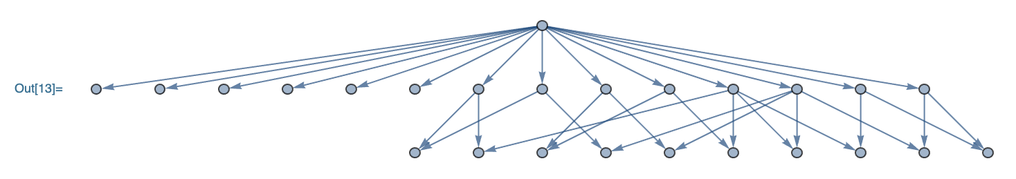
What are the possible ways that five point puzzles from Project L can be solved, with a relative efficiency greater than one? That is it takes shorter than expected in that we can solve the puzzle faster than the puzzle's point value in the top left corner. How do we define units for time? Can we really measure the tile's usefulness by the proportion of puzzle solutions that display the tile?
The dancing links method allows x to exist in a detached state; it continues to exist on a separate linked list from the one at that we are looking such that we can swap it back in for what's left of right (what's right of left). It's going to be fun. Here's my notebook for the tiling of polyominoes.
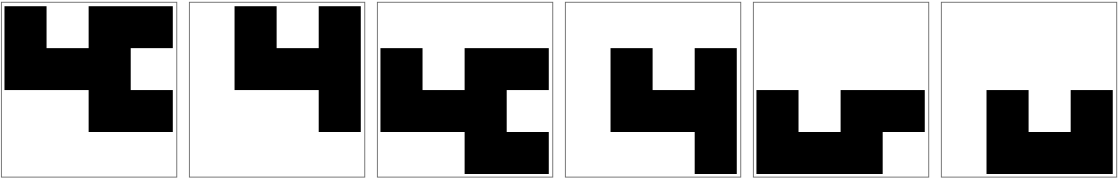
f = {{1, 0, 1, 1}, {1, 1, 1, 0}, {0, 0, 1, 1}};
embeds[f_, {n_, m_}] := Flatten[
   Table[
    ArrayPad[
     f,
     {{i - 1, n - i - Length[f]}, {j - 1, m - j - Length[First[f]]}}
     ],
    {i, n - Length[f] + 1},
    {j, m - Length[First[f]] + 1}
    ], 1];
Grid@Partition[
  ArrayPlot[#,
     ImageSize -> 100] & /@
   embeds[f, {5, 5}], 6]
mirrors[tile_] := Reverse[tile, {2}]
rotates[tile_] := Transpose[Reverse[tile]]
tileSet[tile_] := DeleteDuplicates[
  Join[
   NestList[rotates, tile, 3],
   NestList[rotates, mirrors[tile], 3]
   ]
  ]
tiles = {
   {{1}},
   {{1, 1}},
   {{1, 0}, {1, 1}},
   {{1, 1, 1}}, {{1, 1}, {1, 1}},
   {{0, 1, 0}, {1, 1, 1}},
   {{1, 0, 0}, {1, 1, 1}},
   {{1, 1, 1, 1}}, {{0, 1, 1}, {1, 1, 0}}
   };
tiles = Flatten[tileSet /@ tiles, 1];
myColorFunction = ColorData[{"ArmyColors", "Reversed"}];
enhancedArrayPlot[tile_] := ArrayPlot[
   tile,
   Mesh -> True,
   ImageSize -> 50,
   MeshStyle -> Orange,
   ColorRules -> {
     0 -> Transparent,
     1 -> myColorFunction[RandomReal[]]
     }
   ];
Grid[Partition[enhancedArrayPlot /@ tiles, 14], Frame -> All]
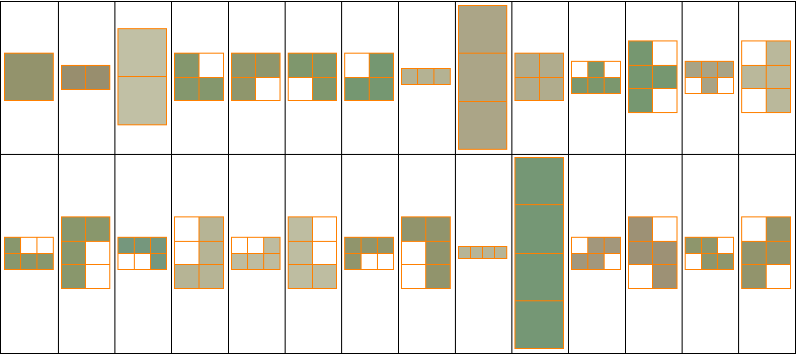
I think this really gets to the crux of Project L which is about solving exact cover problems. The idea is, and I finally see the light now, to use polyomino pieces to complete the puzzles within the given set of constraints. For instance let's say I take my fist, and use that as a unit of measurement to build from the simple description of one fist, and then I build upon that. The puzzle gets big, the constraints get big, and the puzzle gets big..nothing else other than the key component of the strategy game known as Project L, where simple mechanics can build up to a sophisticated discourse on resource management, power, and efficiency.
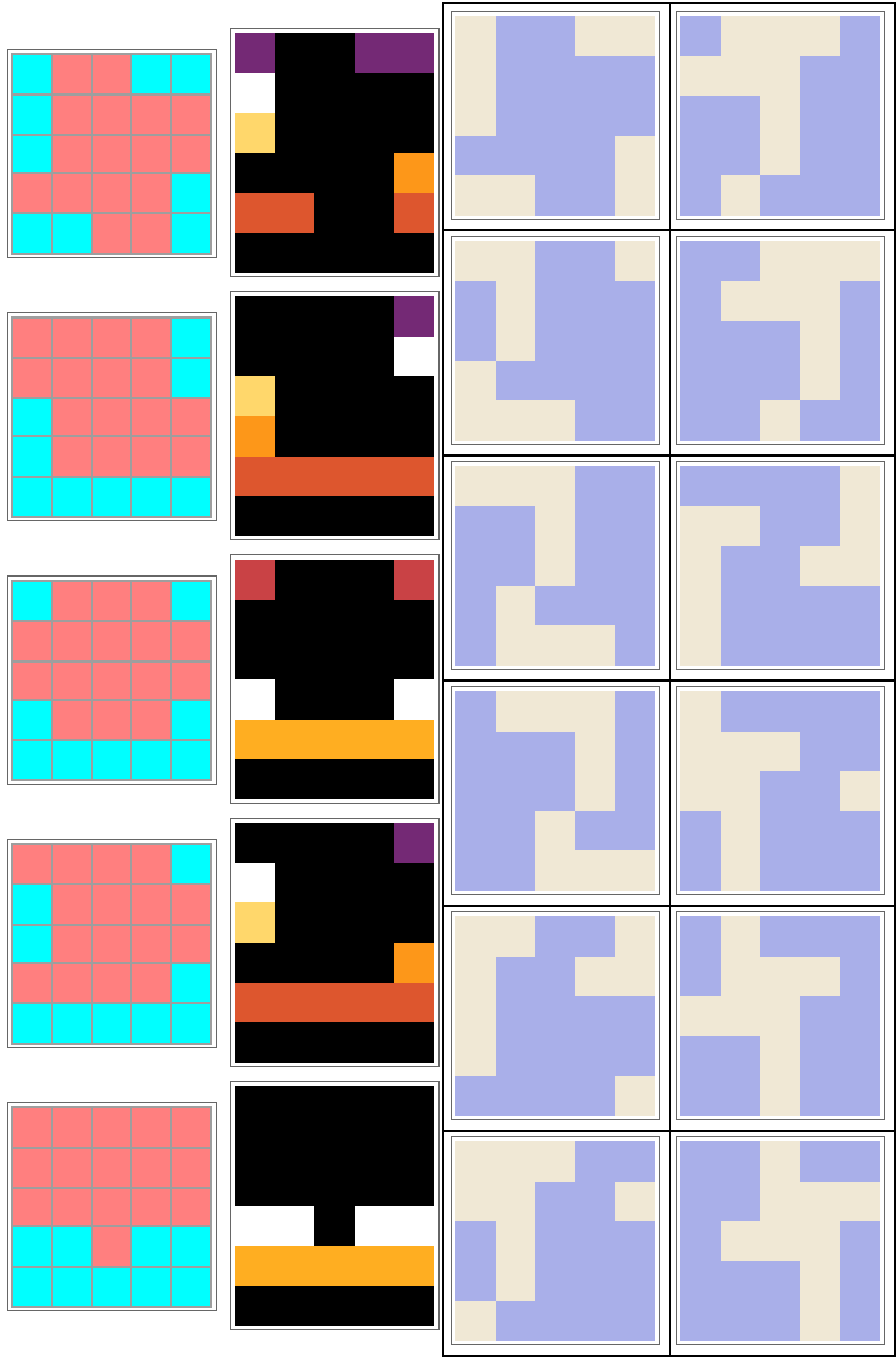
Yes, I know how numpy is the primary foundation of mathematics and computation in Python, whereas in this scenario we're implementing the function of embedding visual representations of the polyominoes and the puzzles, the utility of analyzing piece pseudo-rotations and reflections, and generating possible solutions for tiling puzzles:
rawData = {
   {{1, 0, 0, 1, 1}, {1, 0, 0, 0, 0}, {1, 0, 0, 0, 0}, {0, 0, 0, 0,
     1}, {1, 1, 0, 0, 1}},
   {{0, 0, 0, 0, 1}, {0, 0, 0, 0, 1}, {1, 0, 0, 0, 0}, {1, 0, 0, 0,
     0}, {1, 1, 1, 1, 1}},
   {{1, 0, 0, 0, 1}, {0, 0, 0, 0, 0}, {0, 0, 0, 0, 0}, {1, 0, 0, 0,
     1}, {1, 1, 1, 1, 1}},
   {{0, 0, 0, 0, 1}, {1, 0, 0, 0, 0}, {1, 0, 0, 0, 0}, {0, 0, 0, 0,
     1}, {1, 1, 1, 1, 1}},
   {{0, 0, 0, 0, 0}, {0, 0, 0, 0, 0}, {0, 0, 0, 0, 0}, {1, 1, 0, 1,
     1}, {1, 1, 1, 1, 1}}
   };
VisualizeMatrix[matrix_] := MatrixPlot[matrix,
  Mesh -> All,
  ImageSize -> 100,
  FrameTicks -> None,
  ColorRules -> {1 -> Cyan, 0 -> Pink}
  ]
ShearModal[piece_] := Module[
  {
   dims = Dimensions[piece],
   newArray
   },
  newArray = ArrayPad[
    piece,
    {{0, 1}, {0, 0}}
    ];
  MapIndexed[(#1 /. Rule @@@ Transpose[
        {
         Range[dims[[2]]],
         RotateRight[Range[dims[[2]]], #2[[1]] - 1]
         }
        ]) &, newArray]]
PieceTranslates[piece_, shift_, dims_] := RotateRight[
    PadRight[piece, dims], #] & /@
  Tuples[Range[0, #] & /@ shift]
translation = PieceTranslates[rawData[[1]], {2, 3}, {5, 5}];
Row[{
  Grid[{VisualizeMatrix[#], ArrayPlot[ShearModal[#],
       ColorFunction -> "SunsetColors",
       ImageSize -> 100]} & /@ rawData],
  Grid[Transpose[Partition[MatrixPlot[#,
        ColorFunction -> "LakeColors",
        FrameTicks -> None,
        ImageSize -> 100] & /@
      translation,
     6,
     6,
     {1, 1},
     {}]],
   Frame -> All ]
  }]
Yeah, there's a balance between point value and the utility of reward pieces throughout the gameplay, that's an inherent feature of the game itself where the utility can be mutable. Do we need it to be immutable? Probably not. If you use your imagination the value of a puzzle can be quantified based on these parameters. But why? That would constrain our understanding of the dynamics of multiplayer games and the structure of space-time, which just foreshadows our ability to adapt faster to the future of work.
Considering how the actions of other players could impact individual strategies, there are further choices that can allow us to freely enumerate, for those of us who see these possible plays (and it really does come down to that) for the controlled mini-game version, of Project L, wherein there's a multiway graph and if you look at it from different angles you sort of kind of see that there's neither beginnings nor ends, to the game's complexity and the optimal strategies that we might be able to identify via the timeless computational tutorials on mathematics or the rough introduction to how game analysis works; how can we go beyond intuition to quantify and strategize gameplay?
PieceRotations[_, _][piece_] := {piece}
PartialCoverRows[allowRotation_, allowReflection_][templateMatrix_,
pieceMatrix_] := Module[
{
zeroPositionsInTemplate = Position[templateMatrix, 0],
dimensionsOfTemplate = Dimensions[templateMatrix],
totalOnesInPiece = Total[pieceMatrix, 2],
rotationsAndReflectionsOfPiece,
whichPlacements,
shiftsForPlacement
},
rotationsAndReflectionsOfPiece =
PieceRotations[allowRotation, allowReflection][pieceMatrix];
shiftsForPlacement = Map[
dimensionsOfTemplate - Dimensions[#] &,
rotationsAndReflectionsOfPiece
];
whichPlacements = Catenate[
MapThread[
If[
MemberQ[Sign[#2], -1],
Nothing,
PieceTranslates[#1, #2, dimensionsOfTemplate]
] &,
{
rotationsAndReflectionsOfPiece,
shiftsForPlacement
}]
];
Select[
Outer[#1[[Sequence @@ #2]] &, whichPlacements,
zeroPositionsInTemplate, 1],
Total[#] == totalOnesInPiece &]
]
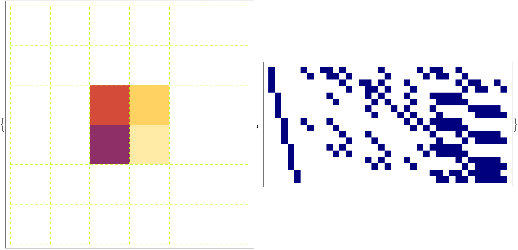
originalMatrix = ArrayPad[ConstantArray[1, {2, 2}], 2, 0];
freshColorFunction = Function[
value,
If[value == 1,
ColorData["SunsetColors"][RandomReal[]],
White]];
limeColor = RGBColor[0.75, 1, 0];
arrayPlotWithFreshColors = ArrayPlot[originalMatrix,
Mesh -> True,
Frame -> True,
ImageSize -> 400,
FrameTicks -> None,
ColorFunction -> freshColorFunction,
MeshStyle -> Directive[limeColor, Dashed]
];
MatricesToCoverMatrix[template_,
pieces_,
OptionsPattern[{
"Rotations" -> True,
"Reflections" -> True,
"PlaceOne" -> False}]] := If[
TrueQ[OptionValue["PlaceOne"]],
Catenate[
MapThread[
Function[{piece, ind},
Join[ind, #] & /@ PartialCoverRows[
OptionValue["Rotations"],
OptionValue["Reflections"]][template, piece]],
{pieces, IdentityMatrix[Length[pieces]]}]],
Catenate[
PartialCoverRows[
OptionValue["Rotations"],
OptionValue["Reflections"]
][template, #] & /@ pieces]]
newMatrix = MatricesToCoverMatrix[
originalMatrix,
rawData,
"PlaceOne" -> True
];
navyColor = RGBColor[0, 0, 0.5];
newPlot = ArrayPlot[newMatrix,
ImageSize -> 400,
ColorRules -> {1 -> navyColor, 0 -> White}
];
{arrayPlotWithFreshColors, newPlot}
When you see things through the lens of exact cover problems, where we've got to use polyominoes - the geometric shapes that could represent things like space weather, or the number of angels that could fit on the needle of a pin, we can fill those specific patterns and puzzles. The Mathematica code can simulate these polyomino pieces so that we can maximize the score wherein the ratio of the puzzle's point value to the actual time taken to solve it, whether we consider each puzzle piece, which doesn't actually exist, to be built up via this metric such that building the polyomino engine shows us how to measure the spending capability of the puzzle, such that we can build upon our backtracking algorithms, heapify them..are we analyzing the game's mechanics deeply enough for our purposes? How can we complete a set of puzzles in the fewest number of turns possible?
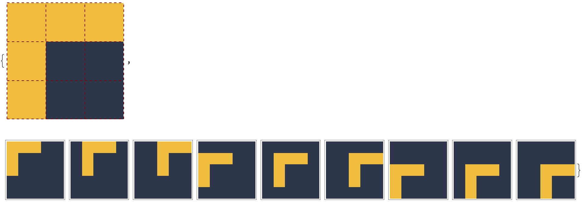
basicPentomino = {{1, 1, 1}, {1, 0, 0}, {1, 0, 0}};
maroonColor = RGBColor[0.5, 0, 0];
arrayPlotPentomino = ArrayPlot[basicPentomino,
   Mesh -> True,
   ImageSize -> 200,
   ColorFunction -> "GrayYellowTones",
   MeshStyle -> Directive[maroonColor, Dashed]
   ];
embedPieceInGrid[piece_, gridDimensions_] := Module[
   {
    pieceDimensions = Dimensions[piece],
    emptyGrid = ConstantArray[0, gridDimensions],
    embeddedGrids
    },
   embeddedGrids = ConstantArray[
     emptyGrid,
     gridDimensions - pieceDimensions + {1, 1}
     ];
   Table[
    embeddedGrids[[row, column]][[row ;;
        row + pieceDimensions[[1]] - 1, column ;;
        column + pieceDimensions[[2]] - 1]] = piece,
    {
     row,
     gridDimensions[[1]] - pieceDimensions[[1]] + 1
     },
    {
     column,
     gridDimensions[[2]] - pieceDimensions[[2]] + 1
     }
    ];
   Flatten[embeddedGrids, 1]];
pentominoEmbeddings = embedPieceInGrid[basicPentomino, {5, 5}];
gridOfArrayPlots = Grid@Partition[
    ArrayPlot[#,
       ImageSize -> Tiny,
       ColorFunction -> "GrayYellowTones"
       ] & /@ pentominoEmbeddings, 9];
{arrayPlotPentomino, gridOfArrayPlots}
Just pretend that a seemingly simple board game like Project L can become a rich subject for proposing how we can find all solutions to a given problem more quickly than the current implementations. It's like when you're bubbling up on a binary tree and want to swap places, to put it lightly we can just represent everything as a matrix of 0s and 1s, so when we get to the end it unfolds in such a way that we have this auspicious doubly linked list which serves as the foundation of the toroidal structure that allows us to join the recursive, depth-first, backtracking algorithm mania wherein every node has to be some special link; the links dance in the sense that nodes can be easily re-moved and reinserted, and we can't help but cover and uncover the rows, the dead ends, and the list structure that gives us an exhaustive search where depth means accuracy and the iterative approach is exponentially complex. And vectorization just recursively solves exact cover problems, when I ask questions and do the Sudoku puzzle research.


