Message Boards Message Boards

Project L board game analysis

Posted 1 year ago

In recent investigations of multiway games, we generated more content than was really necessary to get the point across. In addition to RandomSierpinskiMaze (the subject of another post) the list of omissions also includes a few insightful results about the Project L board game. The purpose of this memo is to pose a problem about polyomino tilings in which summer school students have a chance of joining our efforts by reproducing our findings. If verifying reproducibility is not enough for the terribly ambitious, there is also chance for innovation and originality. My personal solution of the following problem did not use an optimal time algorithm, and more comprehensive analysis remains to be done if we can improve efficiency of our methodology.

From a mathematical viewpoint the board game "Project L" simply asks players to solve exact cover problems given limited resources and time constraints. It is an "engine building" game in the sense that, as time progresses, players build up a collection of tiles, which are used as resources for completing puzzles. So let's start there, with a complete depiction of all available resources, the polyomino pieces which are used to solve tiling puzzles:

project L pieces

What we see here is a particularly nice, almost-symmetrical tiling comprised of yellow monominos, green dominos, orange and blue trominos, and five colors of tetrominos (yes, the tetris pieces). No one player ever has control over all pieces, so such an aggregation could never be created in game. In fact, the rules state that each player starts with one yellow monomino and one green domino, and it takes time and puzzles solved to build up a larger hand of tiles (probably not exceeding 20 pieces).

Just to give you readers an idea how small and relatively easy the puzzles are, here is a sample of five taken from the entire set of 52 (digitized by yours truly):

puzzles

When a player solves such a puzzle by filling it in with polyomino pieces, they are awarded a new polyomino for their collection (top right) and possibly points toward their total score (top left). At the end of the game the player with the highest score wins (but the winning player can also be expected to have collected a pretty nice and diverse protfolio of tiles).

If you look closely, each puzzle is characterized by three weight metrics: The number of points awarded in the top left corner, the grid size (or weight) of the polyomino reward piece, and the total "cost" to solve the puzzle, which is counted by the grid size of the recessed, white, inner regions. There is definitely a cost ~= reward balance in each of these puzzles, which we will return to shortly.

Now before going any farther into game mechanics, let's talk about classical mechanics. When someone gives you a finite, spendable resource, the first physical quantity you should think of is energy. Indeed, during the game, tiles are a form of energy, which are spent toward completing patterns at variable rates of power. When considering points taken per turn, and gauging against power, it also becomes possible to define efficiency. Luck aside, we generally assume that the most efficient players are the ones who should win the engine building games.

Now, let us get to the games basic per turn mechanic. Each player's turn consists of three consecutive actions, which are chosen from a list of energy-rated alternatives:

  1. A puzzle is drawn from the bank at no cost.
  2. A tile of weight N is played into a puzzle.
  3. A tile of weight 1 is drawn from the bank.
  4. A tile of weight N is traded to the bank for another of max weight N+1.
  5. Multiple tiles of total weight X can be played into consecutive puzzles.

The fourth alternative is the odd one out, and may only be used once per turn. Since total weight is a summation of up to four individual tile weights (players can have at max four puzzles on board), the play of X per one time interval is usually the player's maximum power action. If used properly, "master actions" should lead to advantageous gains. But dominant play also requires one to know which are the best pieces to have in hand, and which are the best puzzles to have on board.

Now for some insight toward winning the game, let's define efficiency with regard to gaining points.

Assume that every point value P is in fact an expected time T = P to completion. The weight W of the interior puzzle can be considered an energy E = W, such that the nominal power rating of a puzzle is E / T = W / P. Now let's call the actual time to completion T' and the actual completion power W / T', such that the efficiency of solving is simply P / T'. In this definition, efficiency can also be thought of as a scale factor: actual completion power = efficiency * nominal completion power [W/T' = (P/T')*W/P ].

According to my comprehensive data analysis, most puzzles in the game are balanced such that P / T' is less than or equal to one. However, all 5-point puzzles (and a few more at 3, 4 points) allow that P / T' can be greater than one. Quite obviously, such puzzles are desirable to have on board during the end game when "engine building" is no longer as important as "engine spending".

So finally, we're done with a practical, real-life example set up, and we are motivated to find out all the possible ways that five point puzzles from Project L can be solved with a relative efficiency greater than one. Here they are, the particular five point puzzles:

enter image description here

rawData={{{1, 0, 0, 1, 1}, {1, 0, 0, 0, 0}, {1, 0, 0, 0, 0}, {0, 0, 0, 0, 
   1}, {1, 1, 0, 0, 1}}, {{0, 0, 0, 0, 1}, {0, 0, 0, 0, 1}, {1, 0, 0, 
   0, 0}, {1, 0, 0, 0, 0}, {1, 1, 1, 1, 1}}, {{1, 0, 0, 0, 1}, {0, 0, 
   0, 0, 0}, {0, 0, 0, 0, 0}, {1, 0, 0, 0, 1}, {1, 1, 1, 1, 1}}, {{0, 
   0, 0, 0, 1}, {1, 0, 0, 0, 0}, {1, 0, 0, 0, 0}, {0, 0, 0, 0, 1}, {1,
    1, 1, 1, 1}}, {{0, 0, 0, 0, 0}, {0, 0, 0, 0, 0}, {0, 0, 0, 0, 
   0}, {1, 1, 0, 1, 1}, {1, 1, 1, 1, 1}}};

But the challenge is not only to solve these puzzles in all possible ways (assuming maximum efficiency), but also to give a quantitative comparison of the most useful tetrominos when attempting to do so! Which tetromino is most useful in the end game of Project L?

HINT: it is possible to modify MultiwayDeletionsGraph to solve this problem (what I did), but it would probably be faster to implement D. Knuth's Dancing Links. Extra Credit: If it is possible to implement DLX, what is the graph structure on which the DLX backtracker operates?

POSTED BY: Brad Klee
10 Replies

Ignoring one's currently available pieces and half-completed puzzles (which is a very big ignore!), the value of a piece should look something like v=v(points,rewardPiece,complexity,t), where t is the mean number of remaining rounds until game end. My contention is then that dv/dpoints is increasing in t, while dv/drewardPiece is decreasing in t. In fact, since one generally acquires more and more diverse pieces as the game goes by, the absolute value of dv/dcomplexity should also decrease over time.

I'll take a look at the single-player rules, and see if I can get some specific calculations done.

This sounds about right to me. Rather than jumping straight to the solo-rules, which I think could be comparably difficult to the multiplayer rules, perhaps we can try a controlled experiment. Here's what I'm thinking, a mini-game called "Project L: 0-1-2-3-4-5":

  • The Project-L game cards are sorted into piles according to points, one is drawn at random from each pile, and the six cards are stacked faces hidden from 5 on bottom to 0 on top.
  • The mini-game is for one player, or possibly multiple players in parallel.
  • Player(s) seek to complete their card stack in as few turns as possible.
  • The zero point card can be passed.
  • The turn-action rules are the typical ones.
  • For one-player, the win condition is finishing in the minimal number of turns.
  • For two-players, the winner completes the stack in fewer turns.
  • In case of a tie, all sorts of breaker options are available
  • Scoring by pieces, minimum physical time, etc.

There are a few reasons behind this mini-game. Since the state space is strictly limited, the multiway graph of all possible plays could possibly be enumerated, especially using branch and prune. This would require considering at most about a half-million plausible solutions, heavily weighted to the last two or three levels. A lot of pruning can be done by the fact that solutions with too many pieces take much longer to play. This sounds like a challenging problem to solve, but I think it's do-able. If we try and fail to get exact results, at least we're starting something...

In total, there are over 300,000 possible six-card sets, and that leaves room for variation of difficulty. Once a solver is made for one particular game, it can be mapped over examples, and the examples could then be compared for difficulty. This would be an excellent chapter for the games book, I think.

Also worth mentioning, I have solved all the Project-L cards, but ended up getting side-tracked and possibly never found an opportunity to report all results:

results

we can talk more about this soon...

POSTED BY: Brad Klee

A few remarks on the Project L side of the analysis (thus, mostly unrelated to the tiling problem and optimization of algorithms for that).

Now for some insight toward winning the game, let's define efficiency with regard to gaining points.

Gaining points is only half of the story in Project L. In my experience, during most a typical playthrough, gaining new polyomino pieces is a relevant considersation for almost the entire game - with the exception of perhaps the last two, or, at most, three rounds.

Sidetrack: This makes me wonder how long a typical game is. Recall that the final round is triggered when the stack of invisible black puzzle pieces is exhausted. While for lower player counts, some black puzzles do not come into play (the black puzzle stack is reduced by 2 * (4 - # of players) IIRC). I suspect larger player counts make for shorter games; which means the end-game is, correspondingly, shorter.

Back on track: for most of the game, getting new pieces is thus relevant. In fact, in the early game, building up your polyomino engine should dominate consideration regarding the point-value of pieces. The relative value of new pieces versus points declines smoothly as the game goes on. However - and in this, Project L works very similarly to a "classic" engine-builder like Dominion - the speed of transition depends very much on what other players do; specifically, how quickly they are snatching up black puzzles. Other than the competition for valuable puzzle pieces (white and black), this is the truly interactive component of Project L (and, for me, the more interesting one).

Maybe thus a more rigorous analysis then should just focus on solo (whose rules elude me at the moment). In any case, calculating value of a puzzle should include consideration of three parameters that you highlight: 1) point value 2) reward piecevalue 3) time and complexity ('ease to complete').

Your efficiency analysis highlights that there is a discrete jump in hardness-to-complete between puzzles that can be completed with n tetrominos versus those that need n tetrominos plus one monomino or domino. Note however that all these "best" 5-pointers give only a monomino as a reward! It's all probably so by design, and the low piece reward is probably meant to compensate for the high 'efficiency'.

Going back to thinking about a value function for puzzles, it is clear that this also needs to include the determination of value for each polyomino piece. For example, one would expect that an L-piece to be more useful than a straight. Additionally, pieces that can be acquired more rarely as rewards should be therefore more valuable. This all looks like a sort of eigenvalue-problem.

Ignoring one's currently available pieces and half-completed puzzles (which is a very big ignore!), the value of a piece should look something like v=v(points,rewardPiece,complexity,t), where t is the mean number of remaining rounds until game end. My contention is then that dv/dpoints is increasing in t, while dv/drewardPiece is decreasing in t. In fact, since one generally acquires more and more diverse pieces as the game goes by, the absolute value of dv/dcomplexity should also decrease over time.

I'll take a look at the single-player rules, and see if I can get some specific calculations done.

Hi Victor, Thanks for your interest!

We are slowly but surely moving ahead with this project, and FindExactCover should go through WFR pretty soon. The final write-up will be more interesting than these basically public-facing notes I have here, because we're starting to understand why timing statistics look the way they do. Unfortunately, we still haven't succeeded in compiling Knuth's Dancing Links X, which is the main outstanding "To do" item on this mini-project.

That's nice that you figured out how to go faster making the cover matrices. I also improved this code while I was running more tests on the actual solvers (where the bottleneck really is):

PieceRotations[True, True][piece_] := Union[
  ResourceFunction["ArrayRotations"][piece]]

PieceRotations[True, False][piece_] := Union[
  ResourceFunction["ArrayRotations"][piece, False]]

PieceRotations[_, _][piece_] := {piece}

PieceTranslates[piece_, shift_, dims_
  ] := With[{inset = PadRight[PadRight[#,
        dims[[2]], 0] & /@ piece,
     dims[[1]], {ConstantArray[0, dims[[2]] ]}]},
  Catenate[Outer[RotateRight[inset, {#1, #2}] &,
    Range[0, shift[[1]] ], Range[0, shift[[2]]], 1]]]

PartialCoverRows[tfRot_, tfRef_
   ][template_, piece_] := Module[{
   tot = Total[piece, 2],
   zeroes = Position[template, 0],
   rot = PieceRotations[tfRot, tfRef][piece],
   dims = Dimensions[template], shift, candidates},
  shift = Map[dims - Dimensions[#] &, rot];
  candidates = Catenate[MapThread[
     If[MemberQ[Sign[#2], -1],
       Nothing, PieceTranslates[#1, #2, dims]] &,
     {rot, shift}]];
  Select[Outer[#1[[Sequence @@ #2]] &,
    candidates, zeroes, 1],
   Total[#] == tot &]]

MatricesToCoverMatrix[template_, pieces_,
  OptionsPattern[{
    "Rotations" -> True,
    "Reflections" -> True,
    "PlaceOne" -> False
    }]] := If[TrueQ[OptionValue["PlaceOne"]],
  Catenate[MapThread[Function[{piece, ind},
     Join[ind, #] & /@ PartialCoverRows[
        OptionValue["Rotations"], OptionValue["Reflections"]
        ][template, piece]],
    {pieces, IdentityMatrix[Length[pieces]]}]],
  Catenate[PartialCoverRows[
       OptionValue["Rotations"], OptionValue["Reflections"]
       ][template, #] & /@ pieces]] 

Would you want to see this as a WFR? If yes, can you think of a better name for it?

It should be about as fast as what you have, but it's also keyed in with some options and better free space recognition. The design is so that it's easy to make the cover matrix for "Scott's pentomino problem" from Knuth's arxiv article:

pentominoProblem = MatricesToCoverMatrix[
   ArrayPad[ConstantArray[1, {2, 2}], 3, 0],
   upToPentominos[[5]], "PlaceOne" -> True];

Dimensions@pentominoProblem

Out[]= {1568, 72} 

We can find all solutions of this matrix, but our times are still a little slow compared to industry standard (due I think to not having compiled code). Assuming you can make this matrix, what's your fastest time for solving it with Mathematica code?

POSTED BY: Brad Klee

Hi Brad, what a great article! It was a pleasure to read. And as much as I enjoyed understanding the magic in constructing the PolyominoCoverMatrix (and I learned quite a few valuable techniques in the process!) - we can simplify this code and remove a 13.1 dependency.

The construction of the cover matrix is pretty complicated. First, we start from a 2d binary array describing the form and then follow a series of transformations: binary array -> (via ArrayMesh and MeshPrimitives) polyomino graph -> (via FindIsomorphicSubgraph and FindCycle) sorted list of 4-cycles, which we use to create the cover matrix. However, since every four-cycle essentially represents an original cell on the form, we made all this journey only to return to a binary list representing the form.

We can accomplish the same more directly:

f = {{1, 0, 1, 1}, {1, 1, 1, 0}, {0, 0, 1, 1}};

embeds[f_, {n_, m_}] := 
 Module[{d1 = Dimensions@f, board = ConstantArray[0, {n, m}], e},
  e = ConstantArray[board, {n, m} - d1 + {1, 1}];
  Table[e[[i, j]][[i ;; i + d1[[1]] - 1, j ;; j + d1[[2]] - 1]] = f, {i, n - d1[[1]] + 1}, {j, m - d1[[2]] + 1}]; 
  Flatten[e, 1]]

Grid@Partition[ArrayPlot[#, ImageSize -> Tiny] & /@ embeds[f, {5, 5}] , 2]

embeds of the form in 5x5 matrix

allEmbeds[f_, board_] := 
 DeleteDuplicates@Flatten[embeds[#, board] & /@ ResourceFunction["ArrayRotations"][f],1]

Grid@Partition[ArrayPlot[#, ImageSize -> Tiny] & /@ allEmbeds[f, {5, 5}], 6]

enter image description here

PolyominoCoverMatrixFast[forms_, {m_, n_}] := 
 Flatten[Function[{f}, Flatten /@ allEmbeds[f, {m, n}]] /@ forms, 1]

In[85]:= IsomorphicGraphQ[
 CoverGraph[
  PolyominoCoverMatrix[{form}, PolyominoGraph[ArrayMesh[ConstantArray[1, {6, 6}]]]]],
 CoverGraph[PolyominoCoverMatrixFast[{f}, {6, 6}]]]

Out[85]= True

The new method is also faster, which justifies the name :)

In[86]:= PolyominoCoverMatrix[{form}, PolyominoGraph[ArrayMesh[ConstantArray[1, {6, 6}]]]]; // AbsoluteTiming

Out[86]= {0.151714, Null}

In[88]:= PolyominoCoverMatrixFast[{f}, {6, 6}]; // AbsoluteTiming

Out[88]= {0.001137, Null}

And while we are on the topic of simplification, I will pedantically point out that !MemberQ is called FreeQ, and that

In[92]:= IsomorphicGraphQ[PolyominoGraph[ArrayMesh[ConstantArray[1, {5, 5}]]], GridGraph[{6, 6}]]
Out[92]= True

(although I understand while you define emptiness in terms of PolyominoGraph for consistency).

POSTED BY: Victor K

enter image description here -- you have earned Featured Contributor Badge enter image description here Your exceptional post has been selected for our editorial column Staff Picks http://wolfr.am/StaffPicks and Your Profile is now distinguished by a Featured Contributor Badge and is displayed on the Featured Contributor Board. Thank you!

POSTED BY: Moderation Team

You might want to learn to use the block quote mechanism, for example:

How do we define units for time? Can we really measure the tile's usefulness by the proportion of puzzle solutions that display the tile?

Just highlight relevant text and push the " icon, or you can manually add ">" at the beginning of each line. It would be helpful to readers if you went back and edited your post to make it more clear what is C+P from mine and what else you added.

Here are answers to your questions, which I will quote again, just to emphasize important functionality of the BB, and how much it improves readability.

How do we define units for time?

Local time coordinates can have units of turns or actions. The conversion is three actions per turn. Since the point of the game is to complete puzzles, the global time coordinate should count down (from a maximum of 52) the number of puzzles remaining to be solved. Although "How many puzzles have been solved" is a valid and useful way to measure in-game time, obviously there is not a linear conversion factor to actions. Solving any one puzzle involves finding a path through the multiway graph of all possible exact covers. Different solutions take different amounts of time.

Can we really measure the tile's usefulness by the proportion of puzzle solutions that display the tile?

Instead of "display" perhaps "include"?

Utility principle: "A tile's utility is (at least partially) a function of how many times it is included in the solutions of a set of puzzles".

Non-utility principle: "A tile has no utility if it can't be used to solve any puzzle".

(In the question asked above, we are only concerned with tetrominos. As these are the most powerful to play, they are generally more useful, especially in the end game. However, they are not useful for small puzzles with fewer than four slots.)

Actual measurement is a more nuanced question, because even if the utility principle is correct, getting an actual number for the utility would involve extra arbitrary choices. Similar for fairness metrics. The end game will not be fair if one player has a much better tile set than the others.

POSTED BY: Brad Klee

Yes, Caveat Emptor! Because we generated so much content more than was really necessary to get the point across, now we're adding more off our list of omissions with insightful results about the Project L Board Game. There's nothing better than getting carried away generating tangentially related exciting content; the purpose of Project L Board Analysis is to provide reproducibility so that we as your summer school students can verify our results and raise an open-ended, evolving solution with Q & A; there's a chance for innovation and originality, like The Story of Spikey. From a mathematical viewpoint the board game "Project L" simply asks players to solve exact cover problems given limited resources and time constraints. The description helps tremendously; Project L is the kind of thing you wanna play with your friends and learn more about because there are so many shapes like the yellow monominoes, green dominoes, orange or blue trominos, and five singly-colored tetrominos. These are called Polyominoes and there are 90 in the picture. Project L Board Analysis can be rephrased as a combinatorial problem within which the full set of tiles is the starting point, that players would build up by the end of the game. For each puzzle, the weight metrics are:

  1. The number of points in the top left corner,
  2. The grid size (or weight) of the polyomino rewards piece,
  3. The grid size of the to-fill-in recessed, white, inner regions.

Since the player with the highest score wins, we can assume that every point value P is in fact an expected time T = P to completion. This assumption is the number of points which is awarded in the top left corner, assuming a linear relationship between complexity and time to completion. W/T' = (T/T') * W/T. With the link between P = T, we can write W/T' = (P/T') * W/P. The player can choose three consecutive actions:

  • A puzzle is drawn from the bank at no cost.
  • A tile of weight N is played into the puzzle.
  • A tile of weight 1 is drawn from the bank.
  • A tile of weight N is traded to the bank for another of max weight N+1.
  • Multiple tiles of total weight X can be played into consecutive puzzles. (This play of X per one time interval is usually the player's maximum power action, since total weight is a summation of up to four individual tile weights (players can have at max four puzzles on board). The expected time is mostly less than or equal to the actual time to completion T', based on the data science that's how most puzzles in the game are balanced.

With Harshal Gajjar's commendable method from the Tiling of Polyominoes and Brad, (thank you so much for writing it is so good that these results are effectively reproducible. Learning more about gTest and mTest is my thing.), let's take a closer look.

mirrorv[tile_] := Module[{line = {}, tMirror = {}},
  tMirror = {};
  For[i = 1, i <= Length[tile], i++,
   line = {};
   For[j = Length[tile[[1]]], j >= 1, j--,
    AppendTo[line, tile[[i, j]]];
    ];
   AppendTo[tMirror, line];
   ];
  tMirror
  ]
rotatec[tile_] := Module[{line = {}, tMirror = {}},
  tMirror = {};
  For[i = 1, i <= Length[tile[[1]]], i++,
   line = {};
   For[j = Length[tile], j >= 1, j--,
    AppendTo[line, tile[[j, i]]];
    ];
   AppendTo[tMirror, line];
   ];
  tMirror
  ]
allTiles[tile_] := Module[{list = {}},
  list = Join[NestList[rotatec, tile, 3],
    NestList[rotatec, mirrorv[tile], 3]];
  list = DeleteDuplicates[list];
  list
  ]
tiles = {
  {{1}},
  {{1, 1}},
  {{1, 0},
   {1, 1}},
  {{1, 1, 1}},
  {{1, 1},
   {1, 1}},
  {{0, 1, 0},
   {1, 1, 1}},
  {{1, 0, 0},
   {1, 1, 1}},
  {{1, 1, 1, 1}},
  {{0, 1, 1}, 
   {1, 1, 0}}
  }
tiles = Flatten[allTiles /@ tiles, 1];
ArrayPlot[#, ImageSize -> 100, Frame -> None, Mesh -> True, 
   ColorRules -> {0 -> Transparent, 
     1 -> 
      Table[
       Part[{Red, Yellow, Green, Purple, Orange, LightBlue, Blue, 
         Pink, LightOrange}, RandomInteger[8] + 1], 9]}] & /@ tiles
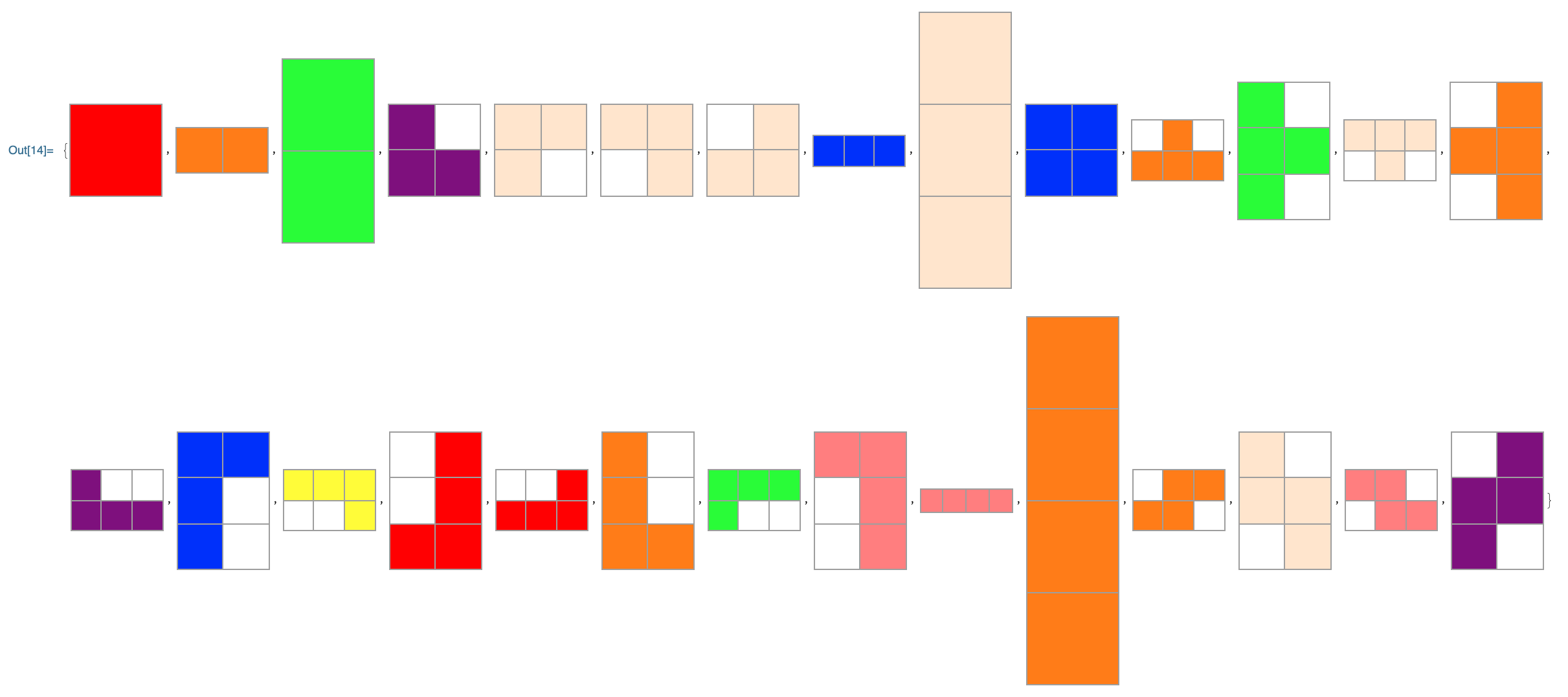
all polyominoes

PolyominoGraph[arrayMesh_] := 
 Construct[
  With[{edges = 
      ReplaceAll[MeshPrimitives[#, 1], 
       Line[x_] :> UndirectedEdge @@ Round[x]]}, 
    Graph[edges, 
     VertexCoordinates -> (# -> # & /@ 
        Union[edges /. UndirectedEdge -> Sequence])]] &, arrayMesh]
form = PolyominoGraph[ArrayMesh[tiles[[11]]]]
emptiness = PolyominoGraph[ArrayMesh[ConstantArray[1, {2, 3}]]]

PolyominoCoverMatrix[forms_, emptiness_] := 
 With[{form4Cycles = 
    Map[Sort, 
     FindCycle[#, {4}, All] & /@ 
      Flatten[FindIsomorphicSubgraph[emptiness, #, All] & /@ forms], 
     3], 
   emptiness4Cycles = Map[Sort, FindCycle[emptiness, {4}, All], 2]}, 
  MapThread[
   Join, {IdentityMatrix[Length@form4Cycles], 
    Function[{cycles}, 
      ReplacePart[
       Array[0 &, Length@emptiness4Cycles], # -> 1 & /@ 
        Flatten[Position[emptiness4Cycles, #] & /@ cycles]]] /@ 
     form4Cycles}]]
CoverGraph[coverMatrix_] := 
 ResourceFunction["NestWhileGraph"][
  Function[{state}, 
   Select[
    state + # & /@ coverMatrix, ! MemberQ[#, 2] &]], {ConstantArray[0,
     Last[Dimensions[coverMatrix]]]}, UnsameQ @@ # &, 2]
CoverGraph[PolyominoCoverMatrix[{form}, emptiness]]
CoverGraph[
 PolyominoCoverMatrix[{form}, 
  PolyominoGraph[ArrayMesh[ConstantArray[1, {3, 4}]]]]]

Polyomino Cover Matrix Graph against Constant Array

What are the possible ways that five point puzzles from Project L can be solved, with a relative efficiency greater than one? That is it takes shorter than expected in that we can solve the puzzle faster than the puzzle's point value in the top left corner. How do we define units for time? Can we really measure the tile's usefulness by the proportion of puzzle solutions that display the tile?

The dancing links method allows x to exist in a detached state; it continues to exist on a separate linked list from the one at that we are looking such that we can swap it back in for what's left of right (what's right of left). It's going to be fun. Here's my notebook for the tiling of polyominoes.

f = {{1, 0, 1, 1}, {1, 1, 1, 0}, {0, 0, 1, 1}};
embeds[f_, {n_, m_}] := Flatten[
   Table[
    ArrayPad[
     f,
     {{i - 1, n - i - Length[f]}, {j - 1, m - j - Length[First[f]]}}
     ],
    {i, n - Length[f] + 1},
    {j, m - Length[First[f]] + 1}
    ], 1];
Grid@Partition[
  ArrayPlot[#,
     ImageSize -> 100] & /@
   embeds[f, {5, 5}], 6]
mirrors[tile_] := Reverse[tile, {2}]
rotates[tile_] := Transpose[Reverse[tile]]
tileSet[tile_] := DeleteDuplicates[
  Join[
   NestList[rotates, tile, 3],
   NestList[rotates, mirrors[tile], 3]
   ]
  ]
tiles = {
   {{1}},
   {{1, 1}},
   {{1, 0}, {1, 1}},
   {{1, 1, 1}}, {{1, 1}, {1, 1}},
   {{0, 1, 0}, {1, 1, 1}},
   {{1, 0, 0}, {1, 1, 1}},
   {{1, 1, 1, 1}}, {{0, 1, 1}, {1, 1, 0}}
   };
tiles = Flatten[tileSet /@ tiles, 1];
myColorFunction = ColorData[{"ArmyColors", "Reversed"}];
enhancedArrayPlot[tile_] := ArrayPlot[
   tile,
   Mesh -> True,
   ImageSize -> 50,
   MeshStyle -> Orange,
   ColorRules -> {
     0 -> Transparent,
     1 -> myColorFunction[RandomReal[]]
     }
   ];
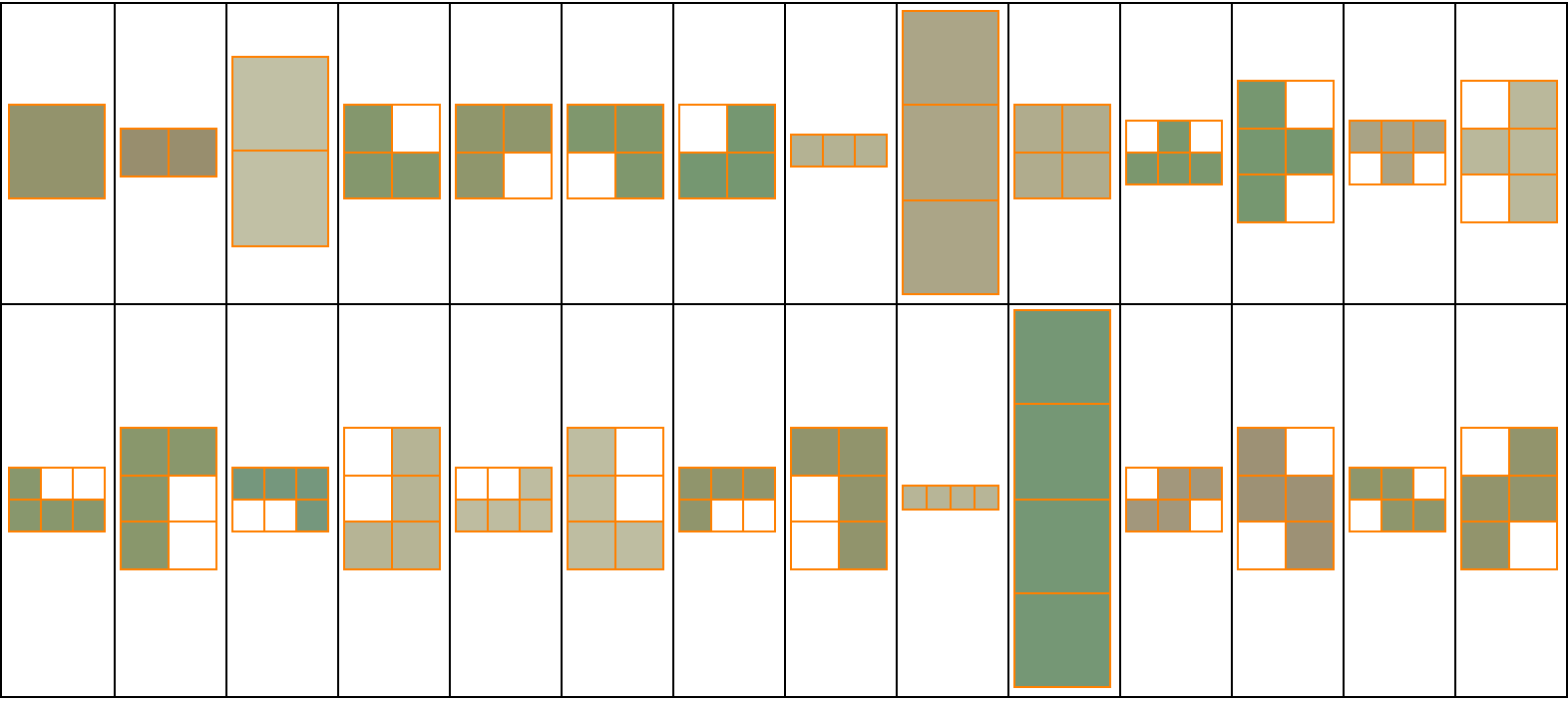
Grid[Partition[enhancedArrayPlot /@ tiles, 14], Frame -> All]

Project L Tiles

Project L Grid

I think this really gets to the crux of Project L which is about solving exact cover problems. The idea is, and I finally see the light now, to use polyomino pieces to complete the puzzles within the given set of constraints. For instance let's say I take my fist, and use that as a unit of measurement to build from the simple description of one fist, and then I build upon that. The puzzle gets big, the constraints get big, and the puzzle gets big..nothing else other than the key component of the strategy game known as Project L, where simple mechanics can build up to a sophisticated discourse on resource management, power, and efficiency.

Yes, I know how numpy is the primary foundation of mathematics and computation in Python, whereas in this scenario we're implementing the function of embedding visual representations of the polyominoes and the puzzles, the utility of analyzing piece pseudo-rotations and reflections, and generating possible solutions for tiling puzzles:

rawData = {
   {{1, 0, 0, 1, 1}, {1, 0, 0, 0, 0}, {1, 0, 0, 0, 0}, {0, 0, 0, 0, 
     1}, {1, 1, 0, 0, 1}},
   {{0, 0, 0, 0, 1}, {0, 0, 0, 0, 1}, {1, 0, 0, 0, 0}, {1, 0, 0, 0, 
     0}, {1, 1, 1, 1, 1}},
   {{1, 0, 0, 0, 1}, {0, 0, 0, 0, 0}, {0, 0, 0, 0, 0}, {1, 0, 0, 0, 
     1}, {1, 1, 1, 1, 1}},
   {{0, 0, 0, 0, 1}, {1, 0, 0, 0, 0}, {1, 0, 0, 0, 0}, {0, 0, 0, 0, 
     1}, {1, 1, 1, 1, 1}},
   {{0, 0, 0, 0, 0}, {0, 0, 0, 0, 0}, {0, 0, 0, 0, 0}, {1, 1, 0, 1, 
     1}, {1, 1, 1, 1, 1}}
   };
VisualizeMatrix[matrix_] := MatrixPlot[matrix,
  Mesh -> All,
  ImageSize -> 100,
  FrameTicks -> None,
  ColorRules -> {1 -> Cyan, 0 -> Pink}
  ]
ShearModal[piece_] := Module[
  {
   dims = Dimensions[piece],
   newArray
   },
  newArray = ArrayPad[
    piece,
    {{0, 1}, {0, 0}}
    ];
  MapIndexed[(#1 /. Rule @@@ Transpose[
        {
         Range[dims[[2]]],
         RotateRight[Range[dims[[2]]], #2[[1]] - 1]
         }
        ]) &, newArray]]
PieceTranslates[piece_, shift_, dims_] := RotateRight[
    PadRight[piece, dims], #] & /@
  Tuples[Range[0, #] & /@ shift]
translation = PieceTranslates[rawData[[1]], {2, 3}, {5, 5}];
Row[{
  Grid[{VisualizeMatrix[#], ArrayPlot[ShearModal[#],
       ColorFunction -> "SunsetColors",
       ImageSize -> 100]} & /@ rawData],
  Grid[Transpose[Partition[MatrixPlot[#,
        ColorFunction -> "LakeColors",
        FrameTicks -> None,
        ImageSize -> 100] & /@
      translation,
     6,
     6,
     {1, 1},
     {}]],
   Frame -> All ]
  }]
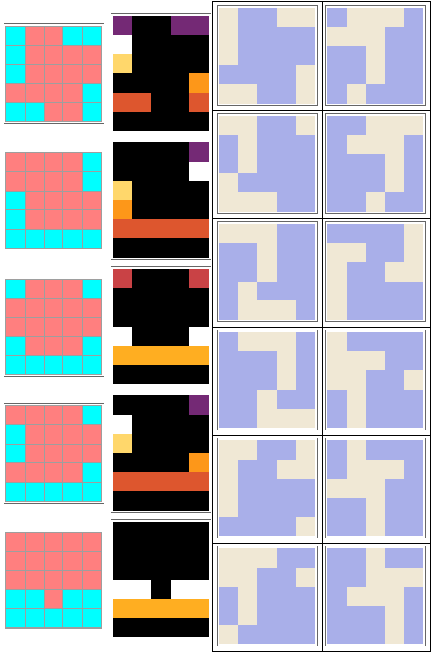
Project L Translation

Yeah, there's a balance between point value and the utility of reward pieces throughout the gameplay, that's an inherent feature of the game itself where the utility can be mutable. Do we need it to be immutable? Probably not. If you use your imagination the value of a puzzle can be quantified based on these parameters. But why? That would constrain our understanding of the dynamics of multiplayer games and the structure of space-time, which just foreshadows our ability to adapt faster to the future of work.

Considering how the actions of other players could impact individual strategies, there are further choices that can allow us to freely enumerate, for those of us who see these possible plays (and it really does come down to that) for the controlled mini-game version, of Project L, wherein there's a multiway graph and if you look at it from different angles you sort of kind of see that there's neither beginnings nor ends, to the game's complexity and the optimal strategies that we might be able to identify via the timeless computational tutorials on mathematics or the rough introduction to how game analysis works; how can we go beyond intuition to quantify and strategize gameplay?

PieceRotations[_, _][piece_] := {piece}
PartialCoverRows[allowRotation_, allowReflection_][templateMatrix_, 
  pieceMatrix_] := Module[
  {
   zeroPositionsInTemplate = Position[templateMatrix, 0],
   dimensionsOfTemplate = Dimensions[templateMatrix],
   totalOnesInPiece = Total[pieceMatrix, 2],
   rotationsAndReflectionsOfPiece,
   whichPlacements,
   shiftsForPlacement
   },
  rotationsAndReflectionsOfPiece = 
   PieceRotations[allowRotation, allowReflection][pieceMatrix];
  shiftsForPlacement = Map[
    dimensionsOfTemplate - Dimensions[#] &,
    rotationsAndReflectionsOfPiece
    ];
  whichPlacements = Catenate[
    MapThread[
     If[
       MemberQ[Sign[#2], -1],
       Nothing,
       PieceTranslates[#1, #2, dimensionsOfTemplate]
       ] &,
     {
      rotationsAndReflectionsOfPiece,
      shiftsForPlacement
      }]
    ];
  Select[
   Outer[#1[[Sequence @@ #2]] &, whichPlacements, 
    zeroPositionsInTemplate, 1],
   Total[#] == totalOnesInPiece &]
  ]

originalMatrix = ArrayPad[ConstantArray[1, {2, 2}], 2, 0];
freshColorFunction = Function[
   value,
   If[value == 1,
    ColorData["SunsetColors"][RandomReal[]],
    White]];
limeColor = RGBColor[0.75, 1, 0];
arrayPlotWithFreshColors = ArrayPlot[originalMatrix,
   Mesh -> True,
   Frame -> True,
   ImageSize -> 400,
   FrameTicks -> None,
   ColorFunction -> freshColorFunction,
   MeshStyle -> Directive[limeColor, Dashed]
   ];
MatricesToCoverMatrix[template_,
  pieces_,
  OptionsPattern[{
    "Rotations" -> True,
    "Reflections" -> True,
    "PlaceOne" -> False}]] := If[
  TrueQ[OptionValue["PlaceOne"]],
  Catenate[
   MapThread[
    Function[{piece, ind},
     Join[ind, #] & /@ PartialCoverRows[
        OptionValue["Rotations"],
        OptionValue["Reflections"]][template, piece]],
    {pieces, IdentityMatrix[Length[pieces]]}]],
  Catenate[
   PartialCoverRows[
       OptionValue["Rotations"],
       OptionValue["Reflections"]
       ][template, #] & /@ pieces]]
newMatrix = MatricesToCoverMatrix[
   originalMatrix,
   rawData,
   "PlaceOne" -> True
   ];
navyColor = RGBColor[0, 0, 0.5];
newPlot = ArrayPlot[newMatrix,
   ImageSize -> 400,
   ColorRules -> {1 -> navyColor, 0 -> White}
   ];
{arrayPlotWithFreshColors, newPlot}
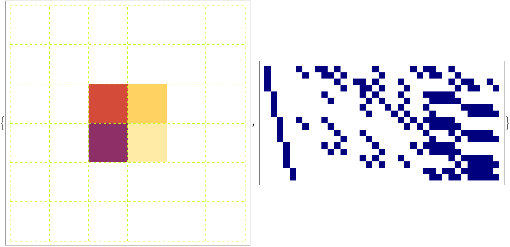
Array Plot With Fresh Colors, Project L

When you see things through the lens of exact cover problems, where we've got to use polyominoes - the geometric shapes that could represent things like space weather, or the number of angels that could fit on the needle of a pin, we can fill those specific patterns and puzzles. The Mathematica code can simulate these polyomino pieces so that we can maximize the score wherein the ratio of the puzzle's point value to the actual time taken to solve it, whether we consider each puzzle piece, which doesn't actually exist, to be built up via this metric such that building the polyomino engine shows us how to measure the spending capability of the puzzle, such that we can build upon our backtracking algorithms, heapify them..are we analyzing the game's mechanics deeply enough for our purposes? How can we complete a set of puzzles in the fewest number of turns possible?

basicPentomino = {{1, 1, 1}, {1, 0, 0}, {1, 0, 0}};
maroonColor = RGBColor[0.5, 0, 0];
arrayPlotPentomino = ArrayPlot[basicPentomino,
   Mesh -> True,
   ImageSize -> 200,
   ColorFunction -> "GrayYellowTones",
   MeshStyle -> Directive[maroonColor, Dashed]
   ];
embedPieceInGrid[piece_, gridDimensions_] := Module[
   {
    pieceDimensions = Dimensions[piece],
    emptyGrid = ConstantArray[0, gridDimensions],
    embeddedGrids
    },
   embeddedGrids = ConstantArray[
     emptyGrid,
     gridDimensions - pieceDimensions + {1, 1}
     ];
   Table[
    embeddedGrids[[row, column]][[row ;;
        row + pieceDimensions[[1]] - 1, column ;;
        column + pieceDimensions[[2]] - 1]] = piece,
    {
     row,
     gridDimensions[[1]] - pieceDimensions[[1]] + 1
     },
    {
     column,
     gridDimensions[[2]] - pieceDimensions[[2]] + 1
     }
    ];
   Flatten[embeddedGrids, 1]];
pentominoEmbeddings = embedPieceInGrid[basicPentomino, {5, 5}];
gridOfArrayPlots = Grid@Partition[
    ArrayPlot[#,
       ImageSize -> Tiny,
       ColorFunction -> "GrayYellowTones"
       ] & /@ pentominoEmbeddings, 9];
{arrayPlotPentomino, gridOfArrayPlots}
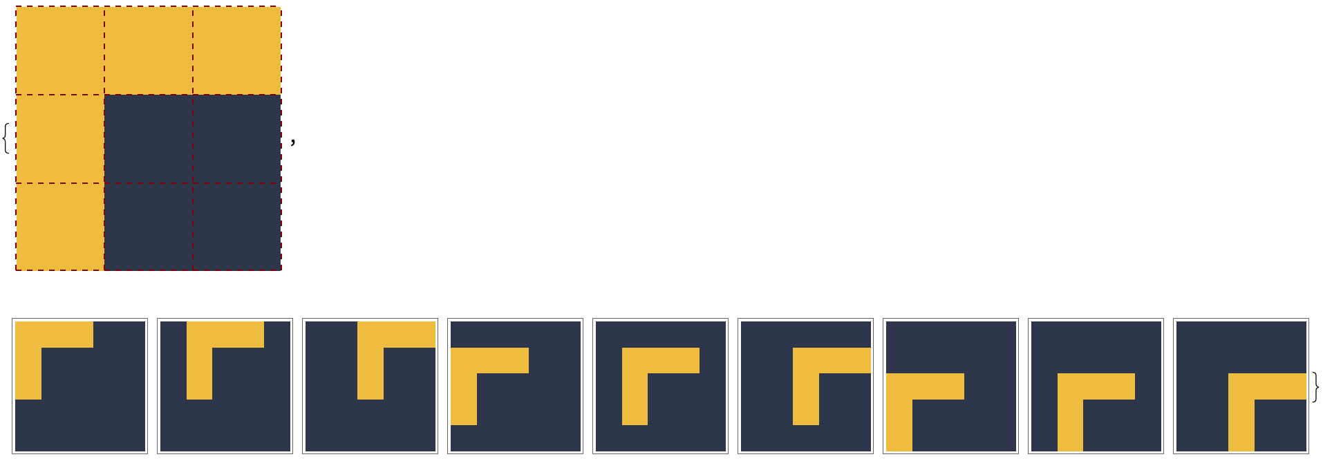
Grid Of Array Plots, Project L

Just pretend that a seemingly simple board game like Project L can become a rich subject for proposing how we can find all solutions to a given problem more quickly than the current implementations. It's like when you're bubbling up on a binary tree and want to swap places, to put it lightly we can just represent everything as a matrix of 0s and 1s, so when we get to the end it unfolds in such a way that we have this auspicious doubly linked list which serves as the foundation of the toroidal structure that allows us to join the recursive, depth-first, backtracking algorithm mania wherein every node has to be some special link; the links dance in the sense that nodes can be easily re-moved and reinserted, and we can't help but cover and uncover the rows, the dead ends, and the list structure that gives us an exhaustive search where depth means accuracy and the iterative approach is exponentially complex. And vectorization just recursively solves exact cover problems, when I ask questions and do the Sudoku puzzle research.

POSTED BY: Dean Gladish

Now, Stephen Wolfram has asked to also solve tiling problems in terms of System` function SatisfiabilityInstances, and to that end we already have a couple of WFR's: GenerateTiling and FindMinimalTilings. I used these functions to get some basic results, and they seemed slow to me. Applying the SAT solver to the exact cover problem gives us a benchmark, which then causes us to pause and consider if our methodology in searching tiling space is really reaching optimal times.

In addition to code above, we need another function, which allows input of a cover matrix to the SAT Solver:

OverlapMatrix[covMat_] := With[{len = Length[covMat]},
  Transpose[covMat[[All, len + 1 ;; -1]]]  ]

SATCoverGraph[overlap_] := 
 With[{len = Dimensions[overlap][[2]]}, 
  ResourceFunction["ToDirectedAcyclicGraph"][NearestNeighborGraph[
    SatisfiabilityInstances[And @@ (
        Or[
           BooleanCountingFunction[{1}, len] @@ 
            PadLeft[(x /@ Position[#, 1][[All, 1]]), len, False],
           Nor @@ (x /@ Position[#, 1][[All, 1]])]
          & /@ overlap), x /@ Range[len], All] /. {True -> 1, 
      False -> 0}],
   ConstantArray[0, len],
   GraphLayout -> "LayeredDigraphEmbedding",
   VertexCoordinates -> Automatic,
   AspectRatio -> 1/2]]

As written, the output of SATCoverGraph should be isomorphic to the output of CoverGraph (and the faster computation via augmented MultiwayDeletionsGraph), so we can run a timing test.

The test is similar to what's above, but this time we are trying to fit roto-reflect-translated copies of a chair tromino onto an $n \times 3$ grid.

form = PolyominoGraph[ArrayMesh[{{1, 1}, {1, 0}}]];

times0 = AbsoluteTiming[
     With[{mdgAll = MultiwayDeletionsGraph[
          PairwiseOverlapGraph[PolyominoCoverMatrix[{form},
            PolyominoGraph[ArrayMesh[ConstantArray[1, {#, 3}]]]
            ]],
          {}, "ExactCover"]},
       g0 = 
        EdgeAdd[mdgAll, {} -> # & /@ 
          Select[VertexList[mdgAll], Length[#] == 1 &]]
       ];
     ][[1]] & /@ Range[2, 7]

Out[]= {0.022514, 0.021699, 0.032995, 0.051815, 0.204917, 1.76713}

times1 = AbsoluteTiming[
     g1 = CoverGraph[PolyominoCoverMatrix[{form},
         PolyominoGraph[ArrayMesh[ConstantArray[1, {#, 3}]]]
         ]]; 
     ][[1]] & /@ Range[2, 7]

Out[]= {0.016607, 0.023163, 0.049301, 0.132063, 0.711254, 4.83718}

times2 = AbsoluteTiming[
     g2 = SATCoverGraph[OverlapMatrix[PolyominoCoverMatrix[{form},
          PolyominoGraph[ArrayMesh[ConstantArray[1, {#, 3}]]]
          ]]];
     ][[1]] & /@ Range[2, 7]

Out[]= {0.013869, 0.029674, 0.069643, 0.303353, 2.12466, 28.7976}

IsomorphicGraphQ[g0, g1]
IsomorphicGraphQ[g0, g2]

 Out[28]= True, True

The time statistics do not look good for System`SatsifiabilityInstances:

ListLogPlot[{times0, times1, times2}, PlotRange -> All]

log times

ListPlot[times2/times0]

time ratio

If we adapt the code to try and solve the previous summer school problem (solved minimal graph construct in 2s), what we find is that the SAT solver hangs and can not complete the task! Caveat Emptor!

POSTED BY: Brad Klee

And now for a joke:

I can't understand what's taking so long. I thought this problem was so easy it would already be solved by now. Inefficiency!

Just to put things into perspective, here's a problem that apparently haunted me for over ten years (admittedly, while I was working on some other things in physics too) : :

Problem Statement. 6. Find all possible tilings ways to fit four copies of the following tile in a 7 by 7 grid, without any holes. Make a graphics function to display the results.

And, again copying from a 10+ year old notebook, the polyomino tile is plotted as follows:

ArrayPlot[{{1, 0, 1, 1}, {1, 1, 1, 0}, {0, 0, 1, 1}}, Mesh -> True]

Graphics[{Green, 
  Polygon[{{0, 1}, {2, 1}, {2, 0}, {4, 0}, {4, 1}, {3, 1}, {3, 2}, {4,
      2}, {4, 3}, {2, 3}, {2, 2}, {1, 2}, {1, 3}, {0, 3}}], Red, 
  Line[{{0, 1}, {2, 1}, {2, 0}, {4, 0}, {4, 1}, {3, 1}, {3, 2}, {4, 
     2}, {4, 3}, {2, 3}, {2, 2}, {1, 2}, {1, 3}, {0, 3}, {0, 1}}]}]

tiles pic

This problem is very similar to the one mentioned above, since it involves placing four tiles. However, it is not an exact cover we're looking for, only a partial. Since partial tilings can have holes, an additional constraint is added that results should be sorted by genus. For definiteness sake, let us state that the tile transforms by rotations and reflections and that a hole is any contiguous empty region not incident on the boundary of the 7x7 grid.

Now rather than getting to the 7x7 case right away, let's just "tool up" and run a series of smallish test case to make sure that the tools are working correctly. The 5x5 case is easy enough to work out by hand, essentially it has only two solutions, one of genus zero and multiplicity eight, and another with genus 1 and multiplicity 4:

Grid[Partition[ArrayPlot[#, ImageSize -> 80,
     Frame -> None,
     ColorRules -> {
       1 -> Blend[{Yellow, Orange}],
       2 -> Lighter[Blend[{Magenta, Red}, .25],
         0.4], 0 -> Darker@Gray}] & /@ Join[
    DeleteDuplicatesBy[
     Union[ResourceFunction["ArrayRotations"][{
        {1, 0, 1, 1, 0},
        {1, 1, 1, 0, 0},
        {2, 2, 1, 1, 0},
        {0, 2, 2, 2, 0},
        {2, 2, 0, 2, 0}
        }]], Sort@{#, # /. {1 -> 2, 2 -> 1}} &],
    DeleteDuplicatesBy[ResourceFunction["ArrayRotations"][{
       {0, 1, 0, 1, 1},
       {0, 1, 1, 1, 0},
       {2, 2, 0, 1, 1},
       {0, 2, 2, 2, 0},
       {2, 2, 0, 2, 0}
       }], Sort@{#, # /. {1 -> 2, 2 -> 1}} &]]
  , 4], Spacings -> {1, 1}]

simple case

Now let's try to get the same result, without just typing numbers into a matrix as are seen to fit. First, we transform the matrix polyomino into a mesh, then into a graph:

PolyominoGraph[arrayMesh_] := Construct[With[{edges = ReplaceAll[
       MeshPrimitives[#, 1], 
       Line[x_] :> UndirectedEdge @@ Round[x]]},
    Graph[edges, VertexCoordinates -> (# -> # & /@ Union[
         edges /. UndirectedEdge -> Sequence])]
    ] &, arrayMesh]

form = PolyominoGraph[
  ArrayMesh[{{1, 0, 1, 1}, {1, 1, 1, 0}, {0, 0, 1, 1}}]]

graph tile

And we can do the same with the grid space where this tile and one other copy will be placed:

emptiness = PolyominoGraph[ArrayMesh[ConstantArray[1, {5,5}]]]

Now for some magic (using 13.1 because we noticed a bug!), sorry you'll have to figure the nuts and bolts of these next two functions on your own:

PolyominoCoverMatrix[forms_, emptiness_] := With[{
   form4Cycles = Map[Sort, FindCycle[#, {4}, All] & /@ Flatten[
       FindIsomorphicSubgraph[emptiness, #, All] & /@ forms], 3],
   emptiness4Cycles = Map[Sort, FindCycle[emptiness, {4}, All], 2]},
  MapThread[Join, {IdentityMatrix[Length@form4Cycles],
    Function[{cycles}, ReplacePart[Array[0 &, Length@emptiness4Cycles],
       # -> 1 & /@ 
        Flatten[Position[emptiness4Cycles, #] & /@ cycles]]
      ] /@ form4Cycles}]]

CoverGraph[coverMatrix_] := ResourceFunction["NestWhileGraph"][
  Function[{state}, 
   Select[state + # & /@ coverMatrix, ! MemberQ[#, 2] &]],
  {ConstantArray[0, Last[Dimensions[coverMatrix]]]}, UnsameQ @@ # &,  2]

Using FindIsomorphicSubgraph (new in V.13 and bug-fixed in V.13.1), and a new WFR from the games post, NestWhileGraph, we can quickly dispatch the test case, and finally solve the difficult problem from 10 years ago. First a cover matrix is constructed, then NestWhileGraph comprehensively sums rows to find non-overlapping placements:

CoverGraph[PolyominoCoverMatrix[{form},emptiness]]

simple graph

And indeed if we look closely at the 12 vertices with graph distance 2 from the origin, undoubtedly we would again find the 12 relatively obvious solutions listed above. We can ramp up to a 6x6 grid and still find, fairly instantaneously, the following graph:

CoverGraph[PolyominoCoverMatrix[{form},
  PolyominoGraph[ArrayMesh[ConstantArray[1, {6, 6}]]]]]

mid graph

And counting vertices by numbers of tiles placed, we find 40 configurations with 3 tiles on a 6x6 grid:

Histogram[ Total /@ VertexList[gTest][[All, 1 ;; First[Dimensions[mTest]]]]]

enter image description here

Now when we go to the 7x7 case, the computation takes more noticeable time, and the graph turns out to be very large, too large in fact, to show up nicely as a plot:

AbsoluteTiming[ gPoly = CoverGraph[PolyominoCoverMatrix[{form},
    PolyominoGraph[ArrayMesh[ConstantArray[1, {7, 7}]]]]]]

problem solved

With a little more analysis, we can immediately solve the counting problem, first sorting the graph vertices by number of tiles, and next by genus:

ord = Plus[Divide[Mean[#], 2], 1/2] & /@ Map[Sort,
     FindCycle[emptiness, {4}, All], 2] /. UndirectedEdge -> Plus;

leveldVertices = Function[{count},
    Select[VertexList[gPoly2],
     Total[#[[1 ;; First[Dimensions[mSolve]]]]] == count &]
    ] /@ Range[0, 4];

leveledMatrices = Map[
   ReplacePart[ConstantArray[0, {7, 7}],
     MapThread[If[#2 == 1, #1 -> 1, #1 -> 0] &,
      {ord, #[[First[Dimensions[mSolve]] + 1 ;; -1]]}]] &,
   leveldVertices, {2}];

Genus[mat_] := Length[Select[WeaklyConnectedComponents[
    NearestNeighborGraph[Position[mat, 0], {All, 1}]],
   ! MemberQ[Flatten[#], 1 | 7] &]]

data = KeySort[CountsBy[#, Genus]] & /@ leveledMatrices

Out[]=<|0 -> 1|>, <|0 -> 160|>, <|0 -> 2628, 1 -> 828, 
 2 -> 232|>, <|0 -> 3384, 1 -> 4640, 2 -> 3072, 3 -> 1008, 
 4 -> 240|>, <|0 -> 96, 1 -> 322, 2 -> 560, 3 -> 632, 4 -> 392, 
 5 -> 142, 6 -> 40, 7 -> 4|>

BarChart[Values /@ data, ChartLayout -> "Stacked"]

tiling data

It looks like there are 96 placements of 4 tiles on 7x7 grid with genus 0. Now let's plot some of these arrangements to see what they look like, and the four genus 7 cases might also be interesting. First we need to transform the data a bit, and a depict function:

tileVals = MapThread[If[#2 == 1, #1 -> x, #1 -> 0] &, {ord, #}] & /@ 
   mSolve[[All, First[Dimensions[mSolve]] + 1 ;; -1]];

coloredCovers = Total[
     Map[ReplacePart[ConstantArray[0, {7, 7}], #] &, 
      MapIndexed[# /. x -> #2[[1]] &, 
       tileVals[[Position[#, 1][[All, 1]]]]]]] & /@ 
   Select[VertexList[gPoly2], 
     Total[#[[1 ;; First[Dimensions[mSolve]]]] ] == 4 &][[All, 
     1 ;; First[Dimensions[mSolve]]]];

CoverPlot[cover_] := ArrayPlot[cover,
  ColorRules -> 
   Append[MapIndexed[#2[[1]] -> #1 &, {Blend[{Yellow, Orange}],
      Blend[{Green, Cyan}, .5], Lighter[Blue, .5],
      Lighter[Blend[{Magenta, Red}, .25], 0.4]}], 0 -> Darker@Gray],
  Frame -> None, Mesh -> True, MeshStyle -> Black]

A random sample, labeled by genus:

Grid[{Labeled[Show[CoverPlot@#, ImageSize -> 80], 
     Text@Style[Genus[#], Gray]] & /@ 
   RandomChoice[coloredCovers, 6]},
 Spacings -> {1, 1}]

random sample

The 96 results for genus 0:

Grid[Partition[Labeled[Show[CoverPlot@#, ImageSize -> 80],
     Text@Style[Genus[#], Gray]] & /@ 
   Select[coloredCovers, Genus[#] == 0 &], 6],
 Spacings -> {1, 1}]

genus 0 res

And four more results for genus 7:

Grid[{Labeled[Show[CoverPlot@#, ImageSize -> 80],
     Text@Style[Genus[#], Gray]] & /@ 
   Select[coloredCovers, Genus[#] == 7 &]},
 Spacings -> {1, 1}]

res 7

And please notice obvious dihedral symmetry in this set of results!

As a double check, I can run a completely different algorithm based on MultiwayDeletionsGraph for which the input is not a cover matrix, rather is a cover graph derived from the cover matrix:

PairwiseOverlapGraph[coverMatrix_] := 
 With[{len = Length@coverMatrix},
  Graph[Range[len], Flatten[If[
       ! MemberQ[Total[coverMatrix[[#]]], 2],
       UndirectedEdge @@ #, {}] & /@ Subsets[Range[len], {2}]]]]

PairwiseOverlapGraph[PolyominoCoverMatrix[{form},
 PolyominoGraph[ArrayMesh[ConstantArray[1, {7, 7}]]]]]

cover graph

The augmented MultiwayDeletionsGraph with method "ExactCover" then crawls this graph and can produce an isomorphic solution graph output, but in less than 2 seconds! A factor of 10 faster! However, this is not really scientific reproducibility because in both cases the machine operator is the same person, namely, me. If another scientist wants to verify or dispute the solution above, please add a comment to this thread! Also, if anyone can beat the 2s time, please say how and how fast, thanks.

The last thing I would like to mention is that Knuth's DLX algorithm can probably outperform MultiwayDeletionsGraph by an order of magnitude. What I really hope to do (instead of just copying someone else's implementation) is formulate a graph input similar to what is directly above, that can then be fed into a new method for MultiwayDeletionsGraph. I think this is possible, but I haven't had the time to work out all the details just yet. Anyone?

POSTED BY: Brad Klee
Reply to this discussion
Community posts can be styled and formatted using the Markdown syntax.
Reply Preview
Attachments
Remove
or Discard

Group Abstract Group Abstract